Deep Background Subtraction with Scene-Specific Convolutional Neural Networks
Department of Electrical Engineering and Computer Science, University of Liège, Belgium
Abstract
Background subtraction is usually based on low-level or hand-crafted features such as raw color components, gradients, or local binary patterns. As an improvement, we present a background subtraction algorithm based on spatial features learned with convolutional neural networks (ConvNets). Our algorithm uses a background model reduced to a single background image and a scene-specific training dataset to feed ConvNets that prove able to learn how to subtract the background from an input image patch. Experiments led on 2014 ChangeDetection.net dataset show that our ConvNet based algorithm at least reproduces the performance of state-of-the-art methods, and that it even outperforms them significantly when scene-specific knowledge is considered.
Keywords: Background subtraction; Deep learning; CDnet; Change detection; Convolutional neural networks; surveillance.
1 Introduction
Detecting moving objects in video sequences acquired with static cameras is essential for vision applications such as traffic monitoring, people counting, and action recognition. A popular approach to this problem is background subtraction, which has been extensively studied in the literature over the last two decades. In essence, background subtraction consists in initializing and updating a model of the static scene, which is named the background (BG) model, and comparing this model with the input image. Pixels or regions with a noticeable difference are assumed to belong to moving objects (they constitute the foreground FG). A complete background subtraction technique therefore has four components: a background initialization process, a background modeling strategy, an updating mechanism, and a subtraction operation.
To address the complexity of dynamic scenes, most researchers have worked on developing sophisticated background models such as Gaussian mixture model
[6], kernel-based density estimation
[1] or codebook construction
[15] (see
[21, 17] for reviews on background subtraction). Other authors have worked on other components such as post-processing operations
[3] or feedback loops to update model parameters (
[15, 16]). In contrast, the subtraction operation is rarely explored. It often consists in a simple probability thresholding operation at the pixel level (
[6, 1]) or in a matching mechanism with collected samples (
[16, 13]). In addition, it is almost exclusively based on low-level features such as color components (
[6, 13]), gradients
[19], or hand-crafted features such as the LBP histogram
[10], LBSP
[16] and matrix covariance descriptor
[20].
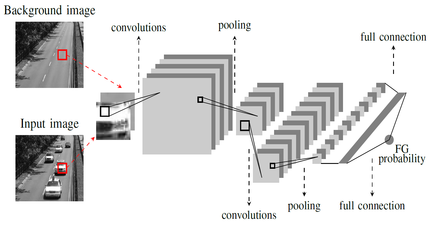
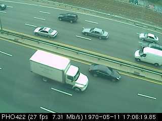
In this work, we show that the complexity of the background subtraction task can be addressed during the subtraction operation itself instead of requiring a complex background modeling strategy. More precisely, we model the background with a single grayscale background image and delegate to a convolutional neural network (ConvNet), trained with a scene-specific dataset, the task of subtracting the background image from the input frame for each pixel location. The process is illustrated in Fig.
1↓. The main benefit of this approach is that ConvNets are able to learn deep and hierarchical features, which turn out to be much more powerful than classical hand-crafted features for comparing image patches. To the best of our knowledge, it is the first attempt to apply convolutional neural networks to the background subtraction problem. Note that this paper is not intended to present a real-time and adaptive technique, but rather to investigate the classification potential of deep features learned with convolutional neural networks for the background subtraction task.
The paper is organized as follows. In Section
2↓, we detail the pipeline of our scene-specific ConvNet based background subtraction algorithm. Section
3↓ describes our experimental set-up and presents comparative results with state-of-the-art methods on the 2014 ChangeDetection.net dataset (CDnet 2014)
[12]. Section
4↓ concludes the paper.
2 ConvNet based background subtraction
Convolutional neural networks (ConvNets) have recently showed impressive results in various vision challenges such as house numbers digit classification
[14], object recognition
[7], and scene labeling
[5]. This is our motivation to challenge ConvNets in the context of background subtraction. The pipeline of our algorithm is presented in Fig.
2↓. It has four parts: (1) background model extraction, (2) scene-specific dataset generation, (3) network training, and (4) ConvNet based background subtraction. These components are described below.
2.1 Background image extraction
Our algorithm models the background with a single grayscale image extracted from a few video frames (we observed that using three color channels only leads to marginal improvements in our case). Input images are therefore also converted from RGB domain to grayscale (named Y hereafter) using the following equation :
We extract a grayscale background image by observing the scene during a short period (150 frames, that is a few seconds, in our experiments) and computing the temporal median
Y value for each pixel. This method is appropriate when the background is visible for at least 50% of the time for each pixel. For cluttered scenes, more sophisticated stationary background estimation methods are needed (see for example
[4]).
2.2 Scene-specific dataset generation
The second step of our pipeline consists in generating a scene-specific dataset that learns the network. Denoting, by
T, the size of the patch centered on each pixel for the subtraction operation (see the red rectangles in Fig.
1↑), a training sample
x is defined as a
Tx
T 2-channel image patch (one channel for the background patch extracted from the median image and one channel for the input patch). The corresponding target value is given by:
where
pc denotes the central pixel of the patch. Note that we normalize all
Y values with respect to the
[0, 1] interval. A sequence of
N fully labeled
Wx
H input images is thus equivalent to a collection of
Nx
Wx
H training samples (assuming that images are zero-padded to avoid border effects). Note that both classes need to be represented in the dataset.
We considered two distinct methods for generating the sequence of fully labeled images :
-
Automatic generation with an existing background subtraction algorithm. The main advantage of this method is that it does not require a human intervention. However, the classification performance of the ConvNet is then upper bounded by the classification performance of the dataset generator.
-
Prior knowledge integration by human expert labeling. This method requires a human expert to annotate input images, but it helps to improve the classification results of the ConvNet significantly. In addition, a few manually labeled images generally suffice to achieve a highly accurate classification result. Therefore, it is a reasonable practical alternative to the time-consuming parameter-tuning process performed when a camera is installed in its new environment.
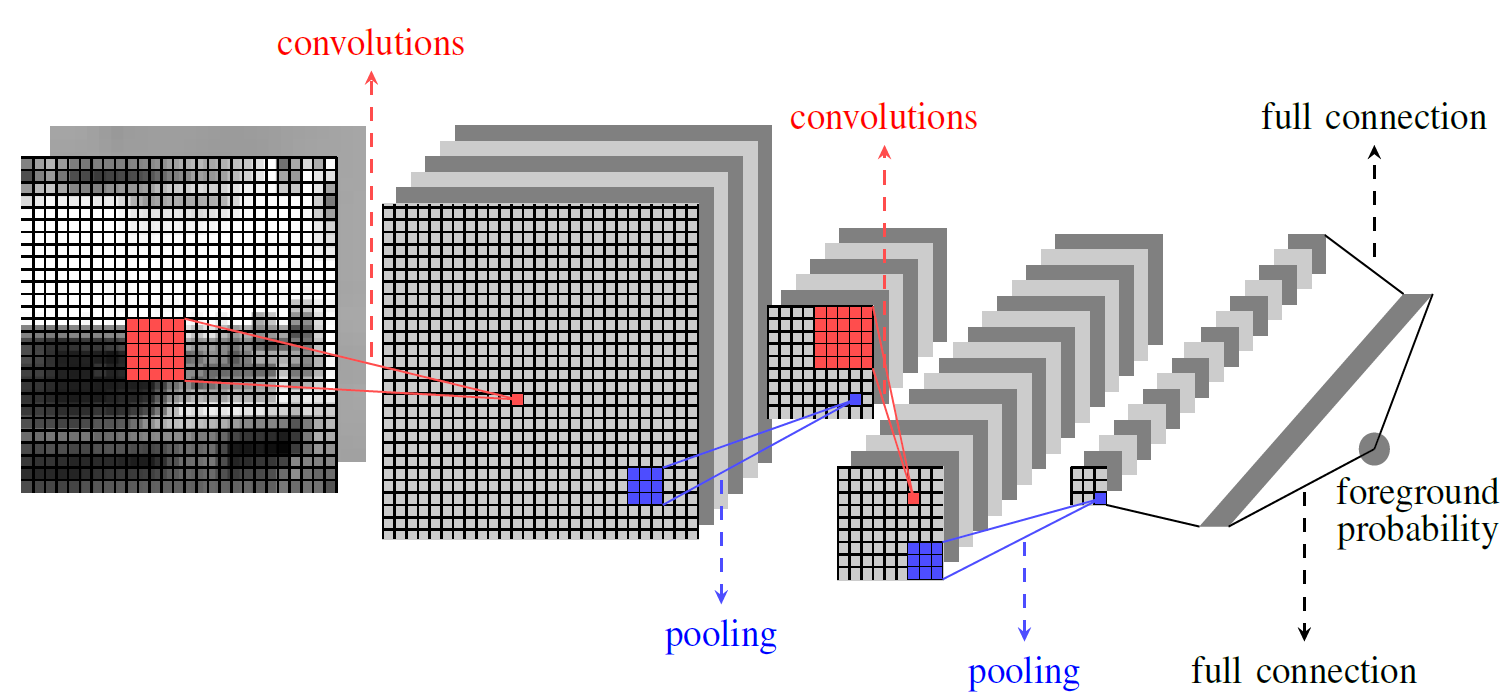
2.3 Network architecture and training
Our ConvNet architecture is showed in Fig.
3↓. It is very similar to
LeNet-5 network for handwritten digit classification
[22], except that subsampling is performed with max-pooling instead of averaging and hidden sigmoid units are replaced with rectified linear units for faster training. It is composed of two feature stages followed by a classical two-layer fully connected feed-forward neural network. Each feature stage consists in a convolutional layer followed by a max-pooling layer. We use a patch size of
T = 27, 5x5 local receptive fields with a 1x1 stride for all convolutional layers (see red patches in Fig.
3↓), and 3x3 non-overlapping receptive fields for all pooling layers (see
blue patches in Fig.
3↓). The first and second convolutional layers have 6 and 16 feature maps, respectively. The first fully connected layer has 120 hidden units and the output layer consists of a single sigmoid unit.
The network contains 20, 243 trainable weights learned by back-propagation with a cross-entropy error function:
where
tn = t(xn), and
yn = p(FG|xn) is the probability that the indexed sample
xn belongs to the foreground. The bias are initially set to
0.1, while other weights are initialized randomly with samples drawn from a truncated normal distribution
N(0, 0.01). Initial values whose magnitude is larger than
0.2 are dropped and re-picked. We use an RMSProp optimization strategy, which gives faster convergence than classical stochastic gradient descent, with a mini-batch size of
100 training samples, and a learning rate of
0.001. The training phase is stopped after
10, 000 iterations.
3 Experimental results
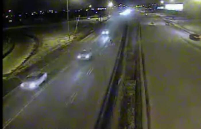
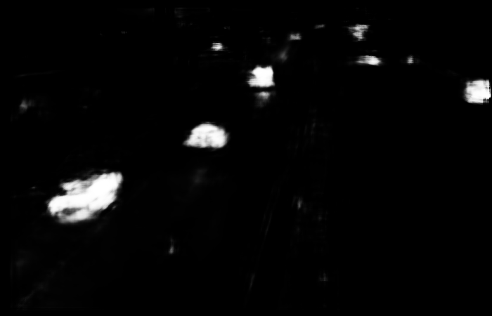
We evaluate our ConvNet based algorithm on the 2014 ChangeDetection.net dataset (CDnet 2014)
[12], which contains real videos captured in challenging scenarios such as camera jitter, dynamic background, shadows, bad weather, night illumination, etc.
Each video comprises a learning phase (no ground truth is available during that phase) and a test phase (ground truth images are given). The first half of test images is used to generate the training data while the second one is used as a test set. To avoid overfitting with respect to the foreground, we restrict our experiments to sequences with different foreground objects between the first and the second halves of the test phase. Table
1↓ provides the list of considered video sequences. Note that PTZ videos have been discarded as our method is specifically designed for static cameras and that videos of the intermittent object motion category does not fulfill our requirement about the foreground.
|
Category
|
Considered videos
|
|
Baseline
|
Highway
|
Pedestrians
|
|
Camera jitter
|
Boulevard
|
Traffic
|
|
Dynamic background
|
Boats
|
Fall
|
|
Shadow
|
Bungalows
|
People In Shade
|
|
Thermal
|
Park
|
|
Bad weather
|
Blizzard
|
Skating
|
Snow fall
|
|
Low framerate
|
Tram crossroad
|
Turnpike
|
|
Night videos
|
all 6 videos
|
|
Turbulence
|
Turbulence 3
|
Table 1 List of videos of CDnet 2014
[12] considered in our experiments
We benchmark our classification results on the test set against those of traditional and state-of-the-art methods reported on the CDnet website, in terms of the F performance metric. This metric represents a trade-off in the precision/recall performance space; it is defined as the harmonic mean of the precision (Pr) and the recall (Re) measures:
It should be as close as possible to 1. It was found in
[12] that the
F measure is well correlated with the ranks of the methods assessed on the CDnet website. We report results for our method trained with data automatically generated with the IUTIS-5 combination algorithm
[18], this variant is denoted by ConvNet-IUTIS, and with ground truth data provided by human experts, this variant is denoted by ConvNet-GT. Results are provided in Table
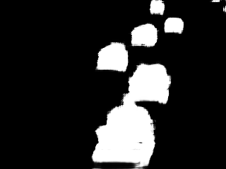
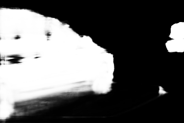
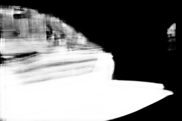
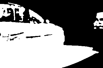
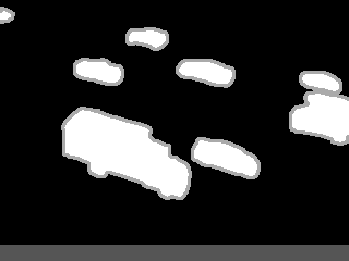
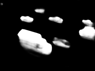
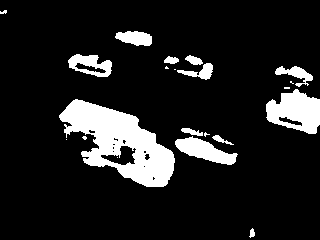
2↓. Fig.
4↓ shows segmentation results of our algorithm as well as for other traditional (GMM
[6] and KDE
[1]), and state-of-the-art (IUTIS-5
[18] and SuBSENSE
[16]) methods.
|
Method
|
Foverall
|
FBaseline
|
FJitter
|
FDynamicBG
|
FShadows
|
FThermal
|
FBadWeather
|
FLowFramerate
|
FNight
|
Fturbulence
|
|
ConvNet-GT
|
0.9046
|
0.9813
|
0.9020
|
0.8845
|
0.9454
|
0.8543
|
0.9264
|
0.9612
|
0.7565
|
0.9297
|
|
IUTIS-5 [18]
|
0.8093
|
0.9683
|
0.8022
|
0.8389
|
0.8807
|
0.7074
|
0.9043
|
0.8515
|
0.5384
|
0.7924
|
|
SuBSENSE [16]
|
0.8018
|
0.9603
|
0.7675
|
0.7634
|
0.8732
|
0.6991
|
0.9195
|
0.8441
|
0.5123
|
0.8764
|
|
PAWCS [15]
|
0.7984
|
0.9500
|
0.8473
|
0.8965
|
0.8750
|
0.7064
|
0.8587
|
0.8988
|
0.4194
|
0.7335
|
|
PSP-MRF [3]
|
0.7927
|
0.9566
|
0.7690
|
0.7982
|
0.8735
|
0.6598
|
0.9135
|
0.8109
|
0.5156
|
0.8368
|
|
ConvNet-IUTIS
|
0.7897
|
0.9647
|
0.8013
|
0.7923
|
0.8590
|
0.7559
|
0.8849
|
0.8273
|
0.4715
|
0.7506
|
|
EFIC [8]
|
0.7883
|
0.9231
|
0.8050
|
0.5247
|
0.8270
|
0.8246
|
0.8871
|
0.9336
|
0.6266
|
0.7429
|
|
Spectral-360 [11]
|
0.7867
|
0.9477
|
0.7511
|
0.7775
|
0.7156
|
0.7576
|
0.8830
|
0.8797
|
0.4729
|
0.8956
|
|
SC_SOBS [9]
|
0.7450
|
0.9491
|
0.7073
|
0.6199
|
0.8602
|
0.7874
|
0.7750
|
0.7985
|
0.4031
|
0.8043
|
|
GMM [6]
|
0.7444
|
0.9478
|
0.6103
|
0.7085
|
0.8396
|
0.7397
|
0.8472
|
0.8182
|
0.4004
|
0.7883
|
|
GraphCut [2]
|
0.7394
|
0.9304
|
0.5183
|
0.7372
|
0.7543
|
0.7149
|
0.9166
|
0.8208
|
0.4751
|
0.7867
|
|
KDE [1]
|
0.7298
|
0.9623
|
0.5462
|
0.5511
|
0.8357
|
0.7626
|
0.8691
|
0.8580
|
0.4057
|
0.7776
|
Table 2 Overall and per-category F scores for different methods (computed for the considered video sequences). Note that averaging F scores might be debatable from a theoretical perspective.
Table
2↑ shows that the quality of our ConvNet based background subtraction algorithm is similar to that of state-of-the-art methods when the training data are generated with IUTIS-5
[18]. When ground truth images are used to generate the training data, our algorithm outperforms all other methods significantly. These results are confirmed in Fig
4↑. In particular, our ConvNet is able to address the unsolved issues of hard shadows and night videos. We found that similar results are obtained when we reduce the number of ground truth images for building the training datasets to 50; it does not affect the quality of the detection. We still get very accurate with 25 images. This shows that ConvNets are a powerful solution for scene-specific background subtraction.
4 Conclusion
In this paper, we present a novel background subtraction algorithm based on convolutional neural networks (ConvNets). Rather than building a sophisticated background model to deal with complex scenes, we use a single grayscale image. However, we improve the subtraction operation itself, by means of a ConvNet trained with scene-specific data. Experimental results on the 2014 CDnet dataset show that our method equals the performance of state-of-the-art methods, or even outperforms them when scene-specific knowledge is provided.
Acknowledgment
References
[1] A. Elgammal, D. Harwood, L. Davis. Non-parametric Model for Background Subtraction. European Conference on Computer Vision (ECCV), 1843:751-767, 2000. URL http://dx.doi.org/10.1007/3-540-45053-X_48.
[2] A. Miron, A. Badii. Change detection based on graph cuts. International Conference on Systems, Signals and Image Processing (IWSSIP):273-276, 2015. URL http://dx.doi.org/10.1109/IWSSIP.2015.7314229.
[3] A. Schick, M. Bauml, R. Stiefelhagen. Improving Foreground Segmentation with Probabilistic Superpixel Markov Random Fields. IEEE International Conference on Computer Vision and Pattern Recognition Workshops (CVPRW):27-31, 2012. URL http://dx.doi.org/10.1109/CVPRW.2012.6238923.
[4] B. Laugraud, S. Piérard, M. Braham, M. Van Droogenbroeck. Simple median-based method for stationary background generation using background subtraction algorithms. International Conference on Image Analysis and Processing (ICIAP), Workshop on Scene Background Modeling and Initialization (SBMI), 9281:477-484, 2015. URL http://dx.doi.org/10.1007/978-3-319-23222-5_58.
[5] C. Farabet, C. Couprie, L. Najman, Y. LeCun. Learning Hierarchical Features for Scene Labeling. IEEE Transactions on Pattern Analysis and Machine Intelligence, 35(8):1915-1929, 2013. URL http://dx.doi.org/10.1109/TPAMI.2012.231.
[6] C. Stauffer, E. Grimson. Adaptive background mixture models for real-time tracking. IEEE International Conference on Computer Vision and Pattern Recognition (CVPR), 2:246-252, 1999. URL http://dx.doi.org/10.1109/CVPR.1999.784637.
[7] C. Szegedy, W. Liu, Y. Jia, P. Sermanet, S. Reed, D. Anguelov, D. Erhan, V. Vanhoucke, A. Rabinovich. Going deeper with convolutions. IEEE International Conference on Computer Vision and Pattern Recognition (CVPR):1-9, 2015. URL http://dx.doi.org/10.1109/CVPR.2015.7298594.
[8] F. Deboeverie G. Allebosch, P. Veelart, W. Philips. EFIC: Edge Based Foreground Background Segmentation and Interior Classification for Dynamic Camera Viewpoints. Advanced Concepts for Intelligent Vision Systems (ACIVS), 9386:130-141, 2015. URL http://dx.doi.org/10.1007/978-3-319-25903-1_12.
[9] L. Maddalena, A. Petrosino. The SOBS algorithm: what are the limits?. IEEE International Conference on Computer Vision and Pattern Recognition Workshops (CVPRW):21-26, 2012.
[10] M. Heikkilä, M. Pietikäinen. A Texture-Based Method for Modeling the Background and Detecting Moving Objects. IEEE Transactions on Pattern Analysis and Machine Intelligence, 28(4):657-662, 2006. URL http://dx.doi.org/10.1109/TPAMI.2006.68.
[11] M. Sedky, M. Moniri, C. Chibelushi. Spectral 360: A physics-based Technique for Change Detection. IEEE International Conference on Computer Vision and Pattern Recognition Workshops (CVPRW):399-402, 2014.
[12] N. Goyette, P.-M. Jodoin, F. Porikli, J. Konrad, P. Ishwar. A Novel Video Dataset for Change Detection Benchmarking. IEEE Transactions on Image Processing, 23(11):4663-4679, 2014. URL http://dx.doi.org/10.1109/TIP.2014.2346013.
[13] O. Barnich, M. Van Droogenbroeck. ViBe: A universal background subtraction algorithm for video sequences. IEEE Transactions on Image Processing, 20(6):1709-1724, 2011. URL http://dx.doi.org/10.1109/TIP.2010.2101613.
[14] P. Sermanet, S. Chintala, Y. LeCun. Convolutional neural networks applied to house numbers digit classification. IEEE International Conference on Pattern Recognition (ICPR):3288-3291, 2012. URL http://ieeexplore.ieee.org/xpl/login.jsp?arnumber=6460867.
[15] P.-L. St-Charles, G.-A. Bilodeau, R. Bergevin. A Self-Adjusting Approach to Change Detection Based on Background Word Consensus. IEEE Winter conference on Applications of Computer Vision (WACV):990-997, 2015. URL http://dx.doi.org/10.1109/WACV.2015.137.
[16] P.-L. St-Charles, G.-A. Bilodeau, R. Bergevin. SuBSENSE: A Universal Change Detection Method with Local Adaptive Sensitivity. IEEE Transactions on Image Processing, 24(1):359-373, 2015. URL http://dx.doi.org/10.1109/TIP.2014.2378053.
[17] P.-M. Jodoin, S. Piérard, Y. Wang, M. Van Droogenbroeck. Overview and Benchmarking of Motion Detection Methods. In Background Modeling and Foreground Detection for Video Surveillance . Chapman and Hall/CRC, Jul 2014. URL http://www.crcnetbase.com/doi/abs/10.1201/b17223-30.
[18] S. Bianco, G. Ciocca, R. Schettini. How Far Can You Get By Combining Change Detection Algorithms?. CoRR, abs/1505.02921, 2015. URL http://arxiv.org/abs/1505.02921.
[19] S. Gruenwedel, P. Van Hese, W. Philips. An Edge-Based Approach for Robust Foreground Detection. Advanced Concepts for Intelligent Vision Systems (ACIVS), 6915:554-565, 2011.
[20] S. Zhang, H. Yao, S. Liu, X. Chen, W. Gao. A covariance-based method for dynamic background subtraction. IEEE International Conference on Pattern Recognition (ICPR):1-4, 2008. URL http://dx.doi.org/.
[21] T. Bouwmans. Traditional and recent approaches in background modeling for foreground detection: An overview. Computer Science Review, 11-12:31-66, 2014. URL http://dx.doi.org/10.1016/j.cosrev.2014.04.001.
[22] Y. LeCun, L. Bottou, Y. Bengio, P. Haffner. Gradient-based learning applied to document recognition. Proceedings of IEEE, 86(11):2278-2324, 1998. URL http://dx.doi.org/10.1109/5.726791.