An Effective Hit-or-Miss Layer Favoring Feature Interpretation as Learned Prototypes Deformations
A. Deliège, A. Cioppa and M. Van Droogenbroeck
University of Liège, Belgium
January 2019
How to cite this work:
A. Deliège, A. Cioppa, and M. Van Droogenbroeck. An Effective Hit-or-Miss Layer Favoring Feature Interpretation as Learned Prototypes Deformations. In AAAI Conference on Artificial Intelligence, Workshop on Network Interpretability for Deep Learning, Honolulu, Hawaii, USA, pages 1-8, January 2019. BiBTeX entry.
Summary
Neural networks designed for the task of classification have become a commodity in recent years. Many works target the development of more effective networks, which results in a complexification of their architectures with more layers, multiple sub-networks, or even the combination of multiple classifiers, but this often comes at the expense of producing uninterpretable black boxes. In this paper, we redesign a simple capsule network to enable it to synthesize class-representative samples, called prototypes, by replacing the last layer with a novel Hit-or-Miss layer. This layer contains activated vectors, called capsules, that we train to hit or miss a fixed target capsule by tailoring a specific centripetal loss function. This possibility allows to develop a data augmentation step combining information from the data space and the feature space, resulting in a hybrid data augmentation process. We show that our network, named
HitNet, is able to reach better performances than those reproduced with the initial CapsNet on several datasets, while allowing to visualize the nature of the features extracted as deformations of the prototypes, which provides a direct insight into the feature representation learned by the network.
1 Introduction
Convolutional neural networks (CNNs) have become an omnipresent tool for image classification and have been revolutionizing the field of computer vision for the last few years. With the emergence of complex tasks such as ImageNet classification
[10], the networks have grown bigger and deeper while regularly featuring new layers and other extensions. This makes it increasingly difficult to understand how the networks make their decisions, which led to the emergence of a new field of research devoted to improve the explainability of neural networks (
\eg [2, 3]). Another usual problem is that CNNs do not generalize well to novel viewpoints because the spatial relationships between different features are generally not preserved in CNNs. Therefore, some models were designed in the spirit of increasing their representational power, hence their interpretability, by encapsulating information in activated vectors called capsules, a notion introduced by Hinton in
[5].
Recent advances on capsules are presented in
[20], in which Sabour
et al. mainly focus on MNIST digits classification
[30]. For that purpose, they develop CapsNet, a CNN that shows major changes compared to conventional CNNs. As described in
[20], “a capsule is a group of neurons whose activity vector represents the instantiation parameters of a specific type of entity such as an object or an object part.” Hence, the concept of capsule somehow adds a (geometrical) dimension to the “capsuled” layers, which is meant to contain richer information about the features captured by the network than in conventional feature maps. The transfer of information from the capsules of a layer to the capsules of the next layer is learned through a dynamic routing mechanism
[9, 20]. The length of the capsules of the last layer, called DigitCaps, is used to produce a prediction vector whose entries are in the
[0, 1] range thanks to an orientation-preserving squashing activation function applied beforehand to each capsule, and which encodes the likelihood of the existence of each digit on the input image. This prediction vector is evaluated through a “margin loss” that displays similarities with the squared hinge loss. In an autoencoder spirit, the capsules encoded in DigitCaps are fed to a decoder sub-network that aims at reconstructing the initial image, which confers the capsules a natural interpretation of the features that they captured. State-of-the-art results are reported by Sabour
et al. in
[20] on MNIST dataset. Other experiments carried out on affNIST
[24], multiMNIST
[20], SVHN
[31], smallNORB
[29] and CIFAR10
[1] (with an ensemble of 7 networks) show promising results as well. Unfortunately, current implementations of CapsNet with dynamic routing are considerably slower to train than conventional CNNs, which is a major drawback of this process.
Since the publication of
[20], several works have been conducted to improve CapsNet’s speed and structure
[4, 9, 18, 26] and to apply it to more complex data
[2, 14, 15] and various tasks:
[25] for localization,
[17] for segmentation,
[3] for reinforcement learning. However, it appears that the attempts (
e.g. [27, 7, 16, 23]) to reproduce the results provided in
[20] failed to reach the reported performances.
Our first contribution is the construction of a neural network, named
HitNet, that provides fast and repeatedly better performances than those reported in
[27, 7, 16, 23] with reproductions of CapsNet by reusing CapsNet’s capsule approach only in one layer, called
Hit-or-Miss layer (HoM, the counterpart of DigitCaps), in a different way. We also provide its associated loss, that we call
centripetal loss (counterpart of the margin loss). Then, we show that plugging the HoM structure into different existing network architectures consistently improves their classification results on various datasets. Finally, we present a way of using the capsules of HoM to derive a hybrid data augmentation algorithm that relies on both real data and synthetic feature-based data by deforming
prototypes, which are class representatives learned indirectly by the decoder.
2 Methods
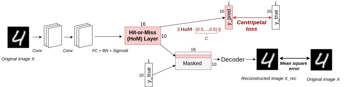
HitNet essentially introduces a new layer, the Hit-or-Miss layer, that is universal enough to be used in many different networks, as shown in the next section.
HitNet as presented hereafter and displayed in Figure
1↑ is thus an instance of a shallow network that hosts this HoM layer and illustrates our point.
The Hit-or-Miss layer
In the case of CapsNet, large activated values are expected from the capsule of DigitCaps corresponding to the true class of a given image, similarly to usual networks. From a geometrical perspective in the feature space, this results in a capsule that can be seen as a point that the network is trained to push far from the center of the unit hypersphere, in which it ends up thanks to the squashing activation function. We qualify such an approach as “centrifugal”. In that case, a first possible issue is that one has no control on the part(s) of the sphere that will be targeted by CapsNet and a second one is that the capsules of two images of the same class might be located far from each other
[22, 32], which are two debatable behaviors.
To circumvent these potential issues, we impose that all the capsules of images of a same class should be located close to each other and in a neighborhood of a given fixed target point. This comes from the hypothesis that all the images of a given class share some class-specific features and that this assumption should also hold through their respective capsules. Hence, given an input image, we impose that HitNet targets the center of the feature space to which the capsule of the true class belongs, so that it corresponds to what we call a hit. The capsules related to the other classes have thus to be sent far from the center of their respective feature spaces, which corresponds to what we call a miss. Our point of view is thus the opposite of Sabour et al.’s; instead, we have a centripetal approach with respect to the true class.
Also, the squashing activation function used by Sabour et al. induces a dependency between the features of a capsule of DigitCaps, in the sense that their values are conditioned by the overall length of the capsule. If one feature of a capsule has a large value, then the squashing prevents the other features of that capsule to take large values as well; alternatively, if the network wishes to activate many features in a capsule, then none of them will be able to have a large value. None of these two cases fit with the perspective of providing strong activations for several representative features as desired in Sabour et al. Besides, the orientation of the capsules, preserved with the squashing activation, is not used explicitly for the classification; preserving the orientation might thus be a superfluous constraint.
Therefore, we replace this squashing activation by a BatchNormalization (BN,
[19]) followed by a conventional sigmoid activation function applied element-wise. We obtain a layer composed of capsules as well that we call the
Hit-or-Miss (HoM) layer, which is
HitNet’s counterpart of DigitCaps. Consequently, all the features obtained in HoM’s capsules can span the
[0, 1] range and they can reach any value in this interval independently of the other features. The feature spaces in which the capsules of HoM lie are thus unit hypercubes.
Defining the centripetal loss
Given the use of the element-wise sigmoid activation, the centers of the reshaped target spaces are, for each of them, the
central capsules C:(0.5, …, 0.5). The
k-th component of the prediction vector
ypred of
HitNet, denoted
ypred, k, is given by the Euclidean distance between the
k-th capsule of HoM and
C:
To give a tractable form to the notions of hits, misses, centripetal approach described above and justify HoM’s name, we design a custom centripetal loss function with the following requirements:
-
The loss generated by each capsule of HoM has to be independent of the other capsules, which thus excludes any probabilistic notion.
-
The capsule of the true class does not generate any loss when belonging to a close isotropic neighborhood of C, which defines the hit zone. Outside that neighborhood, it generates a loss increasing with its distance to C. The capsules related to the remaining classes generate a loss decreasing with their distance to C inside a wide neighborhood of C and do not generate any loss outside that neighborhood, which is the miss zone. These loss-free zones are imposed to stop penalizing capsules that are already sufficiently close (if associated with the true class) or far (if associated with the other classes) from C in their respective feature space.
-
The gradient of the loss with respect to ypred, k cannot go to zero when the corresponding capsule approaches the loss-free zones defined in requirement 2. To guarantee this behavior, we impose a constant gradient around these zones. This is imposed to help the network make hits and misses.
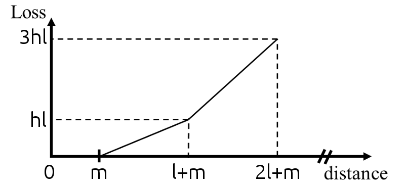
For the sake of consistency with requirement 3, in the present work, we impose piecewise constant gradients with respect to ypred, k, which thus defines natural bins around C, as the rings of archery targets, in which the gradient is constant. Using smoother continuous gradient functions did not seem to have any significant impact.
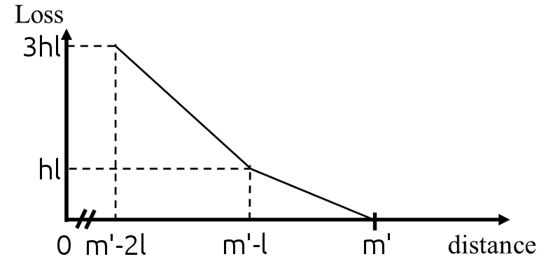
All these elements contribute to define a loss which is a piecewise linear function of the predictions and which is centripetal with respect to the capsule of the true class. We thus call it our centripetal loss. Its derivative with respect to ypred, k is a staircase-like function, which goes up when k is the index of the true class and goes down otherwise. A generic analytic formula of a function of a variable x, whose derivative is an increasing staircase-like function where the steps have length l, height h and vanish on [0, m] is mathematically given by:
where
H{.} denotes the Heaviside step function and
f = ⌊(x − m)/(l)⌋ (
⌊.⌋ is the floor function). Such a function is drawn in Figure
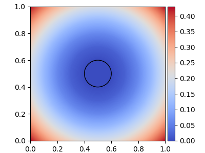
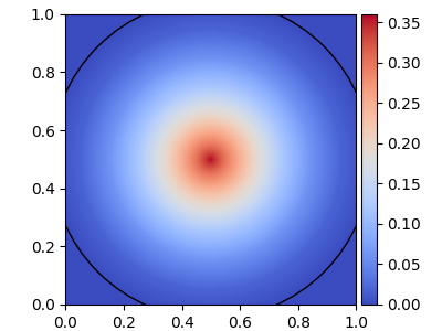
2↓. Hence the loss generated by the capsule of the true class is given by
Ll, h, m(ypred, k), where
k is the index of the true class. The loss generated by the capsules of the other classes can be directly obtained from Equation
2↑ as
Ll’, h’, √(n) ⁄ 2 − m’(√(n) ⁄ 2 − ypred, k’) (for any index
k’ of the other classes) if the steps have length
l’, height
h’, vanish after
m’ and if the capsules have
n components. The use of
√(n) ⁄ 2 originates from the fact that the maximal distance between a capsule of HoM and
C is given by
√(n) ⁄ 2 and thus the entries of
ypred will always be in the interval
[0, √(n) ⁄ 2]. Consequently, the centripetal loss of a given training image is given by
where
K is the number of classes,
yktrue, #2 denotes the
k-th component of the vector
ytrue, and
λ is a down-weighting factor set as
0.5 as in
[20]. The loss associated with the capsule of the true class and the loss associated with the other capsules are represented in Figure
2↓ in the case where
n = 2.
Architecture of HitNet
Basically,
HitNet incorporates a HoM layer built upon feature maps and used in pair with the centripetal loss. We have adopted a shallow structure to obtain these feature maps to highlight the benefits of the HoM layer.
HitNet’s complete architecture is displayed in Figure
1↑. First, it has two
9 × 9 (with strides (1,1) then (2,2)) convolutional layers with
256 channels and ReLU activations, to obtain feature maps. Then, it has a fully connected layer to a
K × n matrix, followed by a BN and an element-wise sigmoid activation, which produces HoM composed of
K capsules of size
n. The Euclidean distance with the central capsule
C:(0.5, …, 0.5) is computed for each capsule of HoM, which gives the prediction vector of the model
ypred. All the capsules of HoM are masked (set to
0) except the one related to the true class (to the predicted class at test time), then they are concatenated and sent to a decoder, which produces an output image
Xrec, that aims at reconstructing the initial image. The decoder consists in two fully connected layers of size
512 and
1024 with ReLU activations, and one fully connected layer to a matrix with the same dimensions as the input image, with a sigmoid activation (this is the same decoder as in
[20]).
If
X is the initial image and
ytrue its one-hot encoded label, then
ytrue and
ypred produce a loss
L1 through the centripetal loss given by Equation
3↑ while
X and
Xrec generate a loss
L2 through the mean squared error. The final composite loss associated with
X is given by
L = L1 + α L2, where
α is set to
0.392 [27, 20]. For the classification task, the label predicted by
HitNet is the index of the lowest entry of
ypred. The hyperparameters involved in
L1 are chosen as
l = l’ = 0.1,
h = h’ = 0.2,
m = 0.1,
m’ = 0.9,
n = 16 and
λ = 0.5 as in
[20].
Prototypes and hybrid data augmentation
In our centripetal approach, we ensure that all the images of a given class will have all the components of their capsule of that class close to 0.5. In other words, we regroup these capsules in a convex space around C. This central capsule C stands for a fixed point of reference, hence different from a centroid, from which we measure the distance of the capsules of HoM; from the network’s point of view, C stands for a capsule of reference from which we measure deformations. In consequence, we can use C instead of the capsule of a class of HoM, zero out the other capsules and feed the result in the decoder: the reconstructed image will correspond to the image that the network considers as a canonical image of reference for that class, which we call its prototype.
After constructing the prototypes, we can slightly deform them to induce variations in the reconstruction without being dependent on any training image, just by feeding the decoder with a zeroed out HoM plus one capsule in a neighborhood of
C. This allows to identify what the features of HoM represent. For the same purpose, Sabour
et al. need to rely on a training image because the centrifugal approach does not directly allows to build prototypes. In our case, it is even possible to compute an approximate range in which the components can be tweaked. If a sufficient amount of training data is available, we can expect the individual features of the capsules of the true classes to be approximately Gaussian distributed with mean
0.5 and standard deviation
m ⁄ √(n). This comes from the BN layer and from Equation
1↑, with the hypothesis that all the values of such a capsule differ from
0.5 from roughly the same amount. Thus the interval
[0.5 − 2m ⁄ √(n), 0.5 + 2m ⁄ √(n)] provides a satisfying overview of the physical interpretation embodied in a given feature of HoM.
The capsules of HoM encode deformations of the prototypes, hence they only capture the important features that allow the network to identify the class of the images and to perform an approximate reconstruction via the decoder. This implies that the images produced by the decoder are not detailed enough to look realistic. The details are lost in the process; generating them back is hard. It is easier to use already existing details, \ie those of images of the training set. We can thus set up a hybrid feature-based and data-based data augmentation process:
-
Take a training image X and feed it to a trained HitNet network.
-
Extract its HoM and modify the capsule corresponding to the class of X.
-
Reconstruct the image obtained from the initial capsule, Xrec, and from the modified one, Xmod.
-
The details of X are contained in X − Xrec. Thus the new (detailed) image is Xmod + X − Xrec. Clip the values to ensure that the resulting image has values in the appropriate range (\eg [0,1]).
3 Experiments and results
Description of the networks used for comparison.
First, we compare the performances of HitNet to three other networks for the MNIST digits classification task. For the sake of a fair comparison, a structure similar to HitNet is used as much as possible for these networks. First, they are made of two 9 × 9 convolutional layers with 256 channels (with strides (1,1) then (2,2)) and ReLU activations as for HitNet. Then, the first network is N1:
-
N1 (baseline model, conventional CNN) has a fully connected layer to a vector of dimension 10, then BN and Softmax activation, and is evaluated with the usual categorical cross-entropy loss. No decoder is used.
The two other networks, denoted N2 and N2b, have a fully connected layer to a 10 × 16 matrix, followed by a BN layer as N1 and HitNet, then
-
N2 (CapsNet-like model) has a squashing activation. The Euclidean distance with O:(0, …, 0) is computed for each capsule, which gives the output vector of the model ypred. The margin loss (centrifugal) of [20] is used;
-
N2b has a sigmoid activation. The Euclidean distance with C:(0.5, …, 0.5) is computed for each capsule, which gives the output vector of the model ypred. The margin loss (centrifugal) of [20] is used.
Network N2b is tested to show the benefits of the centripetal approach of HitNet over the centrifugal one, regardless of the squashing or sigmoid activations. Also, during the training phase, the decoder used in HitNet is also used with N2 and N2b.
Classification results on MNIST.
Each network is trained
20 times during
250 epochs with the Adam optimizer with an initial learning rate of
0.001, with batches of
128 images. The images of a batch are randomly shifted of up to
2 pixels in each direction (left, right, top, bottom) with zero padding as in
[20].
First, the learning rate is kept constant to remove its possible influence on the results. This leads us to evaluate the “natural” convergence of the networks since the convergence is not forced by a decreasing learning rate mechanism. To our knowledge, this practice is not common but should be used to properly analyze the natural convergence of a network.
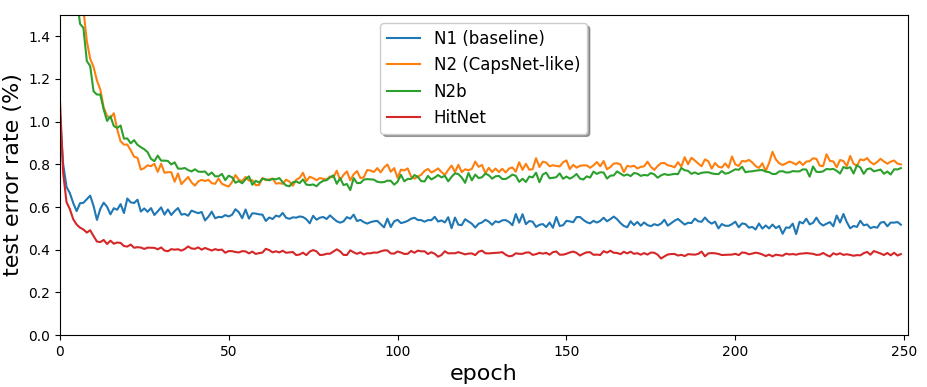
The average test error rates per network throughout the epochs are plotted in Figure
3↓. They clearly indicate that the centripetal approach of
HitNet is better suited than a centrifugal approach. It can also be seen that
HitNet does not suffer from overfitting contrary to N2 and N2b, and that its performance curve appears more “regular” than the others. This indicates that there is an intrinsically better natural convergence associated with
HitNet’s centripetal approach.
The average test error rates at the end of the training are reported in Table
1↓, confirming the superior performances of
HitNet. The associated standard deviations reveal that more consistent results between the runs of a same model (lower standard deviation) are obtained with
HitNet. Let us note that all the runs of
HitNet converged and no overfitting is observed. The question of the convergence is not studied in
[20] and the network is stopped before it is observed diverging in
[16].
|
Network
|
Test error rate (%)
|
|
|
Const./Decr. learning rate
|
Best
|
|
Baseline
|
0.52±0.060 ⁄ 0.42±0.027
|
0.38
|
|
CapsNet-like
|
0.79±0.089 ⁄ 0.70±0.076
|
0.53
|
|
N2b
|
0.76±0.072 ⁄ 0.72±0.074
|
0.62
|
|
HitNet
|
0.38±0.033 ⁄ 0.36±0.025
|
0.32
|
Table 1 Average performance on MNIST test set over the 20 runs of each of the four networks with the associated standard deviation, and single best performance recorded per network.
Then, we run the same experiments but with a decreasing learning rate, to see how the results are impacted when the convergence is forced. The learning rate is multiplied by a factor
0.95 at the end of each epoch. As a result, the networks stabilize more easily around a local minimum of the loss function, improving their overall performances. It can be noted from Table
1↑ that
HitNet is less impacted, which indicates that
HitNet converges to similar states with or without decreasing learning rate. The conclusions are the same as previously:
HitNet performs better. The best error rate obtained for a converged run of each type of network is also indicated in Table
1↑.
Comparisons with reported results of CapsNet on several datasets.
As far as MNIST is concerned, the best test error rate reported in
[20] is
0.25%, which is obtained with dynamic routing and is an average of 3 runs only. However, to our knowledge, the best tentative reproductions reach error rates which compare with our results, as shown in Table
2↓. It is important to underline that such implementations report excessively long training times, mainly due to the dynamic routing part. For example, the implementation
[27] appears to be about
13 times slower than
HitNet, for comparable performances. Therefore,
HitNet produces results consistent with state-of-the art methods on MNIST while being simple, light and fast. For the record, in
[13], authors report a
0.21% test error rate, which is the best performance published so far. Nevertheless, this score is reached with a voting committee of five networks that were trained with random crops, rotation and scaling as data augmentation processes. They achieve
0.63% without the committee and these techniques; if only random crops are allowed (as done here with the shifts of up to 2 pixels), they achieve
0.39%.
The results obtained with
HitNet and those obtained with CapsNet in different sources on Fashion-MNIST
[8], CIFAR10, SVHN, affNIST are also compared in Table
2↓. The architecture of
HitNet described previously is left untouched and the corresponding results reported are obtained with a constant learning rate (excepted for MNIST) and are average test error rates on
20 runs as previously. Some comments about these experiments are given below:
-
Fashion-MNIST: HitNet outperforms reproductions of CapsNet except for [27], but this result is obtained with horizontal flipping as additional data augmentation process.
-
CIFAR10: HitNet outperforms the reproductions of CapsNet. The result provided in [20] is obtained with an ensemble of 7 models. However, the individual performances of HitNet and of the reproductions do not suggest that ensembling them would lead to that result, as also suggested in [28], reporting between 28% and 32% test error rates.
-
SVHN: HitNet outperforms CapsNet from [16], which is the only source using CapsNet with this dataset.
-
affNIST: HitNet outperforms the results provided in [23] and even in Sabour \etal by a comfortable margin. Each image of the MNIST train set is placed randomly (once and for all) on a black background of 40 × 40 pixels, which constitutes the training set of the experiment, and data augmentation is forbidden.. After training, the models are tested on affNIST test set, which consists in affine transformations of MNIST test set.
|
|
|
|
|
|
|
|
et al.
|
0.25
|
-
|
10.60
|
4.30
|
21.00
|
|
et al.
|
0.50
|
10.20
|
32.47
|
8.94
|
-
|
|
|
0.34
|
6.38
|
27.21
|
-
|
-
|
|
|
0.36
|
9.40
|
-
|
-
|
-
|
|
|
0.75
|
10.98
|
30.18
|
-
|
24.11
|
|
|
0.36
|
7.70
|
26.70
|
5.50
|
16.97
|
Table 2 Comparison between the test error rates (in %) reported on various experiments with CapsNet and HitNet, in which case the average results over 20 runs are reported.
HoM with other encoder architectures.
The use of the HoM layer is not restricted to
HitNet, as it can be easily plugged into any network architecture. In this section, we compare the performances obtained on MNIST, Fashion-MNIST, CIFAR10 and SVHN with and without the HoM when the encoder sub-network corresponds to well-known architectures: LeNet-5
[30], ResNet-18
[11] and DenseNet-40-12
[6]. Incorporating the HoM consists in replacing the last fully connected layer (with softmax activation) to a vector of size
K by a fully connected layer to a
K × n matrix, followed by a BN and an element-wise sigmoid activation, which produces HoM composed of
K capsules of size
n. We keep the exact same structure as the one described for
HitNet. As previously, for each dataset, each network is trained from scratch
20 times during
250 epochs, with a constant learning rate and with random shifts of up to
2 pixels in each direction as sole data augmentation process.
The relative decrease in the average test error rates when passing from models without HoM to models with HoM are reported in Table
3↓. The decrease computed from the previous metrics for N1 versus
HitNet is also reported. As it can be seen in Table
3↓, using the HoM layer in a network almost always decreases the test error rates, sometimes by a comfortable margin (
> 15%). As in Figure
3↑, we noticed that the learning curves using the HoM appear much smoother than those from the initial networks. We also noticed that the average standard deviation in the
20 error rates per model is generally lower (
13 experiments among
16) when using the HoM. This metric decreases by at least
20% (and up to
70%) for
9 experiments out of
16, which implies that the use of HoM and the centripetal loss may help producing more consistent results between several runs of a same network.
|
|
MNIST
|
Fash.
|
CIF10
|
SVHN
|
|
N1
|
26.9
|
8.9
|
0.9
|
25.5
|
|
LeNet-5
|
17.3
|
5.3
|
5.9
|
3.9
|
|
ResNet-18
|
20.8
|
7.5
|
8.1
|
17.2
|
|
DenseNet-40-12
|
6.4
|
5.1
|
-0.7
|
15.1
|
Table 3 Relative decrease (in %) in the average test error rates when using the HoM with several architectures.
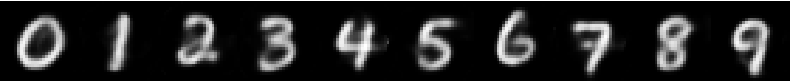
Examining prototypes.
The centripetal approach gives a particular role to the central capsule
C:(0.5, ..., 0.5), in the sense that it can be fed to the decoder to generate prototypes of the different classes. The prototypes obtained from an instance of
HitNet trained on MNIST are displayed in Figure
4↓.
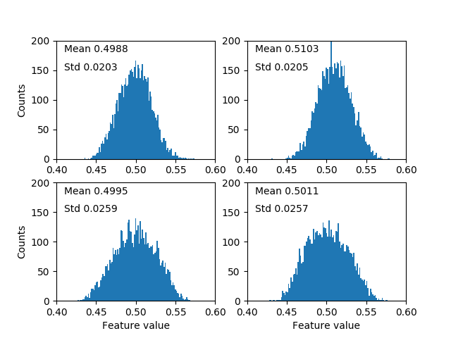
As can be seen in Figure
5↑, the distributions of the individual features of the capsules of the true classes (
\eg capsule 4 for images of the digit “4”) are approximately Gaussian distributed with mean
0.5 and standard deviation
0.1 ⁄ √(16) = 0.025 as explained previously. This confirms that the interval
[0.5 − 2*0.025, 0.5 + 2*0.025] directly provides a satisfying range to visualize the physical interpretation embodied in a given feature of HoM. This is illustrated in Figure
6↑, where one feature of the prototype (in the middle column of each row) is tweaked between
0.45 and
0.55 by steps of
0.01. In our case, in order to visualize the nature of a feature, there is no need to distort real images as in
[20]. As seen in Figure
6↑, on MNIST,
HitNet captures some features that are positional or scale characteristics, others can be related to the width of the font or to some local peculiarities of the digits, as in
[20]. Sampling random capsules close to
C for a given class thus generates new images whose characteristics are combinations of the characteristics of the training images. It thus makes sense to encompass all the capsules of training images of that class in a convex space, as done with
HitNet, to ensure the consistency of the images produced, while CapsNet does not guarantee this behavior. Let us note that, as underlined in
[16], the reconstructions obtained for Fashion-MNIST lacks details and those of CIFAR10 and SVHN are somehow blurred backgrounds; this is also the case for the prototypes. We believe that at least three factors could provide an explanation: the decoder is too shallow, the size of the capsules is too short, and the fact that the decoder has to reconstruct the whole image, including the background, which is counterproductive.
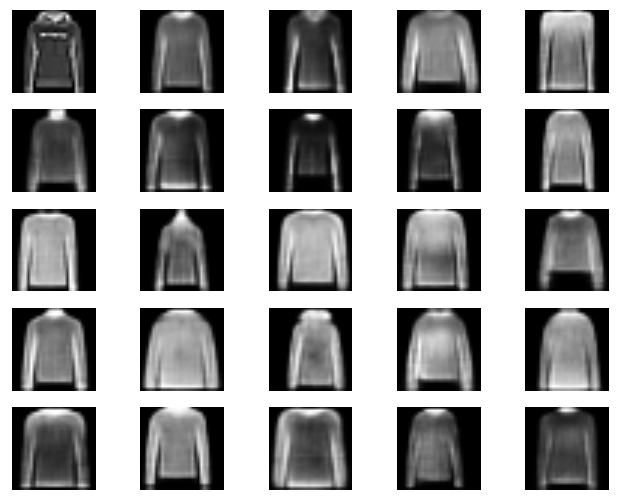
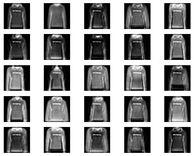
Hybrid data augmentation.
In order to incorporate the details lost in the computation of HoM, the hybrid feature-based and data-based data augmentation technique can be applied. During the step consisting in a modification of the capsules, their values are tweaked of at most
0.025. The importance of adding the details and thus the benefits over the sole data generation process can be visualized in Figure
7↓ with the Fashion-MNIST dataset.
The classification performances can be marginally increased with this data augmentation process as it appeared that networks trained from scratch on such data (continuously generated on-the-fly) perform slightly better than when trained with the original data. On MNIST, the average error rate on 20 models decreased to 0.33% with a constant learning rate and to 0.30% with a decreasing learning rate. In our experiments, 3 of these models converged to 0.26%, one converged to 0.24%. Some runs reached 0.20% test error rate at some epochs. With a bit of luck, a blind selection of one trained network could thus lead to a new state of the art, even though it is known that MNIST digits classification results cannot reach better performances due to inconsistencies in the test set, hence the importance of averaging over many runs to report more honest results. The average test error rate on Fashion-MNIST decreases by 0.2%, on CIFAR10 by 1.5% and on SVHN by 0.2%. These results could presumably be improved with more elaborate encoders and decoders, given the increased complexity of these datasets.
4 Conclusion
We introduce HitNet, a deep learning network characterized by the use of a Hit-or-Miss layer composed of capsules, which are compared to central capsules through a new centripetal loss. The idea is that the capsule corresponding to the true class has to make a hit in its target space, and the other capsules have to make misses. The novelties reside in the reinterpretation and in the use of the HoM layer, which provides new insights on feature interpretability through deformations of prototypes, which are class representatives. These can be used to perform data generation and to set up a hybrid data augmentation process, which is done by combining information from the data space and from the feature space.
In our experiments, we demonstrate that HitNet is capable of reaching state-of-the-art performances on MNIST digits classification task with a shallow architecture and that it outperforms the results reproduced with CapsNet on several datasets, while being at least 10 times faster to train and facilitating feature interpretability. The convergence of HitNet does not need to be forced by a decreasing learning rate mechanism to reach good performances. HitNet does not seem to suffer from overfitting, and provides a small variability in the results obtained from several runs. We also show that inserting the HoM into various network architectures allows to decrease their error rates, which underlies the possible universal use of this layer. It also appears that the results are generally more consistent between several runs of a network when using the HoM, and that the learning curves are more regular. Finally, we show how prototypes can be built as class representatives and we illustrate the hybrid data augmentation process to generate new realistic data. This process can also be used to marginally increase classification performances.
Future work.
The prototypes and all the reconstructions made by the decoder could be improved by using a more advanced decoder sub-network and capsules with more components. In real-life cases such as CIFAR10 and SVHN, it could also be useful to make a distinction between the object of interest and the background. For example, features designed to reconstruct the background only could be used. If segmentation masks are available, one could also use the capsules to reconstruct the object of interest in the segmented image, or simply the segmentation mask. One could also imagine to attach different weights to the features captured by the capsules, so that those not useful for the classification are used in the reconstruction only. The flexibility of HoM allows to implement such ideas easily.
Acknowledgements
We are grateful to M. Braham for introducing us to the work of Sabour et al. and for all the fruitful discussions. This research is supported by the DeepSport project of the Walloon region, Belgium. A. Cioppa has a grant funded by the FRIA, Belgium.
References
[1] A. Krizhevsky: Learning Multiple Layers of Features from Tiny Images. 2009. Technical report, University of Toronto.
[2] P. Afshar, A. Mohammadi, K. Plataniotis: “Brain Tumor Type Classification via Capsule Networks”, CoRR, 2018. URL https://arxiv.org/abs/1802.10200.
[3] P.-A. Andersen: “Deep Reinforcement Learning using Capsules in Advanced Game Environments”, CoRR, 2018. URL https://arxiv.org/abs/1801.09597.
[4] M. Bahadori: “Spectral Capsule Networks”, International Conference on Learning Representations (ICLR), 2018. URL https://openreview.net/forum?id=HJuMvYPaM. Withdrawn paper.
[5] G. Hinton, A. Krizhevsky, S. Wang: “Transforming Auto-Encoders”, International Conference on Artificial Neural Networks (ICANN), pp. 44-51, 2011. URL http://doi.org/10.1007/978-3-642-21735-7_6.
[6] G. Huang, Z. Liu, L. van der Maaten, K. Weinberger: “Densely Connected Convolutional Networks”, IEEE International Conference on Computer Vision and Pattern Recognition (CVPR), pp. 2261-2269, 2017. URL http://doi.org/10.1109/CVPR.2017.243.
[7] H. Liao: CapsNet-Tensorflow. GitHub, 2018. URL https://github.com/naturomics/CapsNet-Tensorflow.
[8] H. Xiao, K. Rasul, R. Vollgraf: “Fashion-MNIST: a Novel Image Dataset for Benchmarking Machine Learning Algorithms”, CoRR, 2017. URL https://arxiv.org/abs/1708.07747.
[9] G. Hinton, S. Sabour, N. Frosst: “Matrix capsules with EM routing”, International Conference on Learning Representations (ICLR), 2018. URL https://openreview.net/forum?id=HJWLfGWRb.
[10] J. Deng, W. Dong, R. Socher, L. Li, K. Li, L. Fei-Fei: “ImageNet: A Large-Scale Hierarchical Image Database”, IEEE International Conference on Computer Vision and Pattern Recognition (CVPR), pp. 248-255, 2009. URL http://doi.org/10.1109/CVPR.2009.5206848.
[11] K. He, X. Zhang, S. Ren, J. Sun: “Deep Residual Learning for Image Recognition”, CoRR, 2015. URL https://arxiv.org/abs/1512.03385.
[12] L. Perez, J. Wang: “The Effectiveness of Data Augmentation in Image Classification using Deep Learning”, CoRR, 2017. URL https://arxiv.org/abs/1712.04621.
[13] L. Wan, M. Zeiler, S. Zhang, Y. Le Cun, R. Fergus: “Regularization of Neural Networks using DropConnect”, International Conference on Machine Learning (ICML), pp. 1058-1066, 2013. URL http://proceedings.mlr.press/v28/wan13.html.
[14] Y. Li, M. Qian, P. Liu, Q. Cai, X. Li, J. Guo, H. Yan, F. Yu, K. Yuan, J. Yu, L. Qin, H. Liu, W. Wu, P. Xiao, Z. Zhou: “The recognition of rice images by UAV based on capsule network”, Cluster Computing, pp. 1-10, 2018. URL https://doi.org/10.1007/s10586-018-2482-7.
[15] J. O'Neill: “Siamese Capsule Networks”, CoRR, 2018. URL https://arxiv.org/abs/1805.07242.
[16] P. Nair, R. Doshi, S. Keselj: Pushing the Limits of Capsule networks. Technical note, 2018.
[17] R. Lalonde, U. Bagci: “Capsules for Objects Segmentation”, CoRR, 2018. URL https://arxiv.org/abs/1804.04241.
[18] D. Rawlinson, A. Ahmed, G. Kowadlo: “Sparse Unsupervised Capsules Generalize Better”, CoRR, 2018. URL https://arxiv.org/abs/1804.06094.
[19] S. Ioffe, C. Szegedy: “Batch Normalization: Accelerating Deep Network Training by Reducing Internal Covariate Shift”, International Conference on Machine Learning (ICML), pp. 448-456, 2015.
[20] S. Sabour, N. Frosst, G. Hinton: “Dynamic Routing Between Capsules”, CoRR, 2017. URL https://arxiv.org/abs/1710.09829.
[21] S. Wong, A. Gatt, V. Stamatescu, M. McDonnell: “Understanding Data Augmentation for Classification: When to Warp?”, Digital Image Computing: Techniques and Applications, pp. 1-6, 2016. URL http://doi.org/10.1109/DICTA.2016.7797091.
[22] A. Shahroudnejad, A. Mohammadi, K. Plataniotis: “Improved Explainability of Capsule Networks: Relevance Path by Agreement”, CoRR, 2018. URL https://arxiv.org/abs/1802.10204.
[23] T. Shin: CapsNet-TensorFlow. GitHub, 2018. URL https://github.com/shinseung428/CapsNetTensorflow.
[24] T. Tieleman: affNIST. https://www.cs.toronto.edu/~tijmen/affNIST/, 2013. URL https://www.cs.toronto.edu/~tijmen/affNIST/.
[25] W. Liu, E. Barsoum, J. Owens: “Object Localization and Motion Transfer learning with Capsules”, CoRR, 2018. URL https://arxiv.org/abs/1805.07706.
[26] D. Wang, Q. Liu: “An Optimization View on Dynamic Routing Between Capsules”, International Conference on Learning Representations (ICLR), 2018. URL https://openreview.net/forum?id=HJjtFYJDf.
[27] X. Guo: CapsNet-Keras. GitHub, 2017. URL https://github.com/XifengGuo/CapsNet-Keras.
[28] E. Xi, S. Bing, Y. Jin: “Capsule Network Performance on Complex Data”, CoRR, 2017. URL https://arxiv.org/abs/1712.03480.
[29] Y. LeCun, Fu Jie Huang, L. Bottou: “Learning methods for generic object recognition with invariance to pose and lighting”, IEEE International Conference on Computer Vision and Pattern Recognition (CVPR), pp. 97-104, 2004. URL http://doi.org/10.1109/CVPR.2004.1315150.
[30] Y. Lecun, L. Bottou, Y. Bengio, P. Haffner: “Gradient-based learning applied to document recognition”, Proceedings of IEEE, pp. 2278-2324, 1998. URL http://doi.org/10.1109/5.726791.
[31] Y. Netzer, T. Wang, A. Coates, A. Bissacco, B. Wu, A. Ng: “Reading Digits in Natural Images with Unsupervised Feature Learning”, Advances in Neural Information Processing Systems (NIPS), 2011.
[32] L. Zhang, M. Edraki, G.-J. Qi: “CapProNet: Deep Feature Learning via Orthogonal Projections onto Capsule Subspaces”, CoRR, 2018. URL https://arxiv.org/abs/1805.07621.