A new jump edge detection method for 3D cameras
A. Lejeune, S. Piérard, M. Van Droogenbroeck, J. Verly
INTELSIG Laboratory, Montefiore Institute, University of Liège, Belgium
December 2011
PDF version of this document
 --- BiBTeX entry
Abstract
Edges are a fundamental clue for analyzing, interpreting, and understanding 3D scenes: they describe objects boundaries. Available edge detection methods are not suited for 3D cameras such as the Kinect or a time-of-flight camera: they are slow and do not take into consideration the characteristics of the cameras. In this paper, we present a fast jump edge detection technique for 3D cameras based on the principles of Canny’s edge detector. We first analyze the characteristics of the range signal for two different kinds of cameras: a time-of-flight camera (the PMD[vision] CamCube) and the Kinect. From this analysis, we define appropriate operators and thresholds to perform the edge detection. Then, we present some results of the developed algorithms for both cameras.
1 Introduction
Edge detection is one of the fundamental techniques in image processing to extract features from an image. Generally, an edge represents a discontinuity in the value of an image. For grayscale images, under common assumption about the image formation process, an edge may correspond to a discontinuity in depth, surface orientation, reflectance or illumination
[10]. With a depth map or a range image, the uncertainty about the physical nature of the edge is lifted: we only have depth discontinuities. In the literature, these edges are often called
jump edges. They are of particular importance since they correspond to boundaries of surfaces and objects. In addition, another type of edges is often defined for range images. These edges correspond to the discontinuities in the first derivative, or equivalently in the surface normals or in the surface orientation. They are called
roof or
crease edges. In this paper, we don’t consider this type of edges.
First, we briefly present existing edge detection methods for range images and explain why they are not suited to the cameras we consider. Then, we start from a standard method of edge detection, the Canny edge detector, and adapt it to our needs. We show that the assumption made on the noise by Canny is no longer valid for range images. Then, we derive a new edge detection operator that takes into account the uncertainty related to any depth value. Finally, we present results for our new edge detector.
1.1 Related work
There already exist edge detection methods for range images. They usually consider both jump and roof edges simultaneously. Most techniques try to fit a model on a substructure of the image to accurately compute the derivatives. Parvin
et al. [2] fit a third-order polynomial on the neighborhood of each pixel to compute the first and second derivatives. Jiang
et al. [11] split each line of the image into a set of quadratic polynomials. Approaches using mathematical morphology operators have also been developed
[7, 8]. More recently, Coleman
et al.\etal
[9] have developed a Laplacian operator for irregular grids to extract edges in range images. A simple criterion was used by Steder
et al.\etal
[3] for detecting jump edges only. All these methods generally present good results on relatively simple scenes.
However, all these techniques were designed and tested for range images captured by laser ranging devices with no concern for real-time performance since the acquisition itself is not in real-time. Also, they do not take into account the differences between each acquisition techniques and how the 3D data is obtained. Recently, real-time 3D acquisition has been made possible with time-of-flight cameras or the Kinect.
1.2 Canny’s edge detector
The basis of our algorithm is the procedure used for the computation of Canny’s edge detector
[4]. It is one of the most successful algorithms developed for edge detection in grayscale images. By assuming an additive white Gaussian noise in images, Canny derived an optimal operator for edge detection that can be approximated by the derivatives of a Gaussian. The method can be be summarized in four steps:
-
Noise reduction by smoothing the image.
-
Computation of the gradient.
-
Removal of non maximum values.
-
Hysteresis thresholding.
The two first steps implement a Gaussian derivative filter. First, noise is reduced in the image by convolving it with a Gaussian filter. Its standard deviation σfilter is a parameter of the method. Then, a derivative operator is applied to the smoothed image I(x, y) for each axis. This yields the gradient ∇I(x, y) at each pixel of the image. Any derivative operator can be used, such as a central difference or a Sobel operator.
The next step of the algorithm is to locate the pixels that are maxima of the gradient magnitude ∥∇I(x, y)∥ along the gradient of the pixel itself and to mark those pixels as possible edges. This is called non-maximum suppression because the algorithm eliminates edge points that aren’t maxima. The last step, hysteresis thresholding, uses two thresholds over the gradient magnitude to only select strong edges. The two thresholds τinf < τsup are used sequentially. First, all maxima pixels that have a gradient magnitude over the biggest threshold τsup are marked as edge pixels. Then, the algorithm recursively selects all locations with a gradient magnitude larger than τinf that are adjacent to an edge pixel as edges themselves
A raw application of Canny’s algorithm on a range image captured by a time-of-flight camera or a Kinect doesn’t yield good results (see Figure
1↑). Indeed, the algorithm assumes the same error distribution for every pixel in the image and 3D images captured with these cameras have an error distribution that changes with each pixel.
1.3 Overview of the proposed method
In this paper, given a range image
D(x, y), we argue that the two thresholds
τinf and
τsup should be adapted according to the uncertainty on
∥∇D(x, y)∥(which is related to the noise level). Here, the uncertainty on a measurement is defined as the standard deviation of the random variable that is sampled. Within a grayscale image, this uncertainty is constant, but this is not the case for range cameras. We propose to use two adaptive thresholds defined as
τ’inf
=
τinf + ασ∥∇D(x, y)∥
τ’sup
=
τsup + ασ∥∇D(x, y)∥
where
α is a parameter of the algorithm, and
σ∥∇D(x, y)∥ is the uncertainty on
∥∇D(x, y)∥. However, in order to take this uncertainty into account also in the non-maximum suppression step of Canny’s algorithm, we prefer computing an adapted value of the gradient magnitude instead of correcting the thresholds
∥∇D(x, y)∥adapted = ∥∇D(x, y)∥ − ασ∥∇D(x, y)∥.
To estimate the uncertainty on
∥∇D(x, y)∥, we start by characterizing two typical range cameras (the Kinect and the PMD[vision] CamCube) in Section
2↓. Then, in Section
3↓, we show how
σ∥∇D(x, y)∥ is computed as a function of the uncertainty on the distance measurements.
2 Sensor characterization
Our goal is to determine the precision, or reciprocally the standard deviation, of each measurement made by the cameras. It is an important characteristic of the signal. It allow us to develop a better criterion for detecting edges. In the next two subsections, we briefly describe the acquisition process of both cameras and derive approximate laws for how the precision may vary inside a single range image.
2.1 Kinect
The Kinect can be seen as a stereoscopic camera. The part of the device responsible for depth acquisition is composed of an infrared illumination source and an infrared camera. The emitted illumination pattern is considered as the right image of a stereoscopic rig. The pattern provides a texture to every surface present in the scene. It is a matter of computing correspondences between the emitted pattern and its observation to recover depth.
Assuming that the disparity is a random variable following a normal distribution, Khoshelham
[5] showed that the standard deviation of the depth
D for the Kinect is:
where
κkinect is a constant of proportionality which depends on several camera parameters and the standard deviation of the disparity.
2.2 Time-of-flight cameras
A time-of-flight camera derives the depth from the time of flight (round trip time) of an electromagnetic signal between the camera and the scene. In our experiment, we have used a PMD (Photonic Mixer Device) camera
[12]. It works by recovering the phase shift between the emitted signal, which is modulated, and the received signal. These cameras provide three channels:
-
The distance d between the camera and the corresponding point in the scene.
-
The amplitude A, which measures the strength of the signal used to compute d. The amplitude is an indicator of the accuracy of the distance measurement.
-
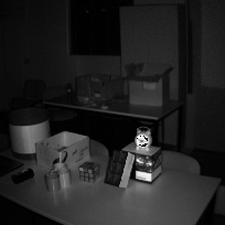
The intensity I, which measures the amount of light received by the sensor. It is similar to a grayscale image captured by a 2D camera.
The depth precision depends on a multitude of factors including the depth, the surface orientation, and reflectance properties. Nevertheless, Frank
et al. [6] propose a good approximation of the standard deviation of a distance measurement, expressed as
where
κcamcube is a constant of proportionality. The precision increases with the amplitude of the signal. It should be noted that, for short distances or with long integration time, the measurements are also unreliable because of a saturation effect in the sensor. The integration time of the camera must be chosen accordingly to the considered application so that the amplitude is maximized without any saturation effect. It must be noted that the amplitude is inversely proportional to the squared depth for the same surface properties and orientation.
2.3 Edge characterization
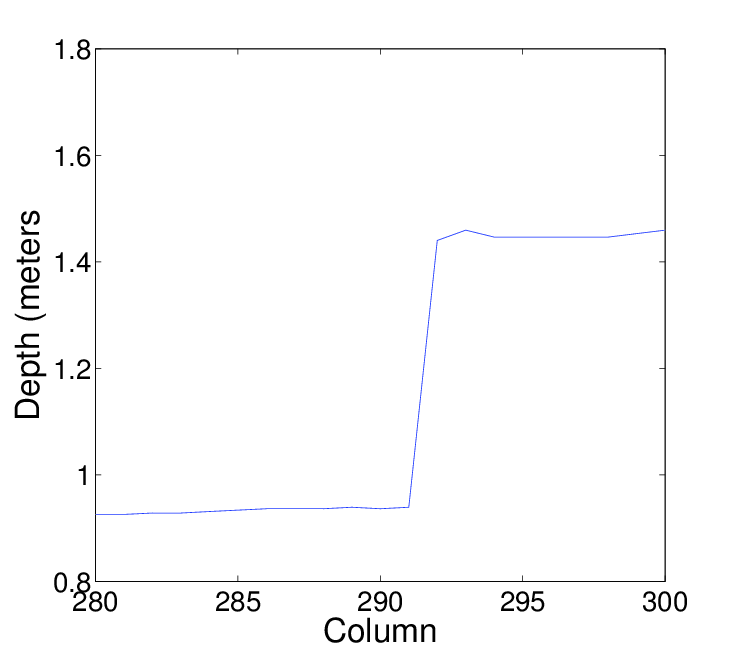
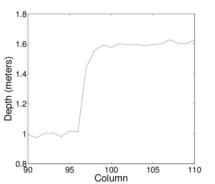
Jump edges represent depth discontinuities. Depending on the method used to capture 3D information, an edge can have different physical meanings. Indeed, each range image pixel corresponds to a solid angle. Thus, the real surface represented by a single pixel depends on the depth and orientation of the surface itself. According to the method used to capture the 3D information, the depth can be sampled on a single point of the solid angle or averaged over the whole surface. So, if a depth discontinuity is present inside the solid angle corresponding to a pixel, its depth may be a mixture of the depth from both sides of the edge. Moreover, the farther the scene is, the larger the surface over which the depth is averaged will be.
We have observed that the PMD[vision] CamCube time-of-flight camera displays noisy jump edges with pixels sampled from both sides of the physical edge. On the other hand, the Kinect gives clean edges. This means that the discontinuity in depth is always located between two pixels and does not spread over several intermediate pixels. An example of jump edges for both cameras is shown in Figure
2↓.
3 Jump edge detection
Since the error on depth may vary for each pixel, we have to adapt a step in Canny’s procedure. The depth values are only used during the second step, the gradient computation. So, we adapt the gradient magnitude to the level of uncertainty of the depth values used to compute it. To achieve this, we derive an upper bound on the standard deviation of the gradient magnitude and define a new adaptive gradient magnitude.
Let
D be a range image and
D(x, y) denote the depth at location
(x, y). We denote the image derivatives along its first and second coordinates as
Dx(x, y) and
Dy(x, y). The gradient is defined by
∇D(x, y) = (Dx(x, y), Dy(x, y)) and its magnitude by the Euclidean norm:
To shorten notations, we will skip the coordinates (x, y) of the pixel unless there is a possible ambiguity. In the following developments, we assume that pixel values are correlated (ρ = 1) if pixels are located on the same surface and independent (ρ = 0) if pixels are separated by a jump edge.
For now, let us assume that the standard deviation of the derivatives,
σDx and
σDy, are known. Their covariance is equal to zero since the derivatives in the two orthogonal directions are independent. Therefore, we can express the standard deviation of the gradient magnitude as
[1]:
σ∥∇D∥2 = ||(∂∥∇D∥)/(∂Dx)||2σDx2 + ||(∂∥∇D∥)/(∂Dy)||2σDy2
with
(∂∥∇D∥)/(∂Dx) = (Dx)/(∥∇D∥).
So, we obtain
σ∥∇D∥
≤ σ∥∇D∥*
= (|Dx|σDx + |Dy|σDy)/(∥∇D∥).
To simplify the developments in the following, we use the upper bound
σ∥∇D∥* instead of the standard deviation of the gradient magnitude
σ∥∇D∥ The standard deviation of the derivatives depends on the operator used to compute them. This operator is usually a linear combination of the values of the pixel and of some neighbors. Using the general equation
Dx(x, y) = ⎲⎳(u, v) ∈ N(x, y)c(u, v)D(u, v),
where
N(x, y) is the neighborhood used to compute the derivative and
c(u, v) the coefficients of the derivative operator, we can compute an upper bound to its standard deviation (see the appendix):
For example, for the forward difference,
Dx(x, y) = D(x + 1, y) − D(x, y),
we have:
σDx(x, y) ≤ σD(x + 1, y) + σD(x, y).
Now that we have derived a general upper bound for the standard deviation of the gradient magnitude, we can use it to adapt Canny’s hysteresis thresholding technique:
∥∇D∥ > τi + ασ∥∇D∥ i = inf, sup.
This criteria means that the gradient magnitude must be larger than a threshold plus a certain amount of its standard deviation to be an edge. From this expression, we define the adaptive gradient magnitude:
∥∇D∥adapted = ∥∇D∥ − ασ∥∇D∥
In the last equation, we adjust the gradient magnitude according to its standard deviation. In addition, we have introduced another parameter in the method,
α. In the implementation, it also includes the proportionality constant
κ used in Section
2↑ to define the standard deviation of the depth.
From this general procedure, we describe our edge detection algorithm for the Kinect and PMD[vision] CamCube cameras. We also make some observations on the data that leads to simplification of the edge detector for the Kinect.
3.1 Kinect
As explained in Section
2.3↑, depth discontinuities in the images captured by the Kinect are clean. This means that we can obtain a single high response in the gradient magnitude by choosing the appropriate derivative operator. A forward or backward difference operator yields a single high value at the pixel preceding or following the edge. In our implementation of the algorithm, we have used a forward difference. Using such a simple derivative filter permits to compute the exact position of the edge.
Using the derivatives, we compute the adaptive gradient magnitude:
∥∇D(x, y)∥adapted = ∥∇D(x, y)∥
− (α)/(∥∇D(x, y)∥)(|Dx(x, y)|(D2(x, y) + D2(x + 1, y))
+ |Dy(x, y)|(D2(x, y) + D2(x, y + 1))) .
We have noticed that the non-maximum suppression step is unnecessary with the Kinect. Indeed, the device is unable to compute the depth on surface that have a high gradient. Thus, using appropriate thresholds τinf and τsup, the pixels having a gradient magnitude superior to them can be considered as edge pixels. The suppression of this step speeds up the algorithm as we avoid at least two comparisons for each pixel. There is no need to apply any other noise reducing method prior to the computation of the gradient. Its adapted version is robust enough to avoid it.
3.2 Time-of-flight cameras
The edges are harder to detect with a time-of-flight camera. The complete algorithm requires all the steps of Canny’s edge detector. First, we smooth the range image with a Gaussian. Then, we compute the derivatives with a central difference. Thus, the adaptive gradient magnitude is given by:
∥∇D(x, y)∥adapted = ∥∇D(x, y)∥
− (α)/(∥∇D(x, y)∥)⎛⎝|Dx(x, y)|⎛⎝(1)/(A(x − 1, y)) + (1)/(A(x + 1, y))⎞⎠
+ |Dy(x, y)|⎛⎝(1)/(A(x, y − 1)) + (1)/(A(x, y + 1))⎞⎠⎞⎠ .
The non-maximum suppression must be applied before performing the hysteresis thresholding. The thresholds are determined experimentally, according to the integration time and the captured scene.
4 Results
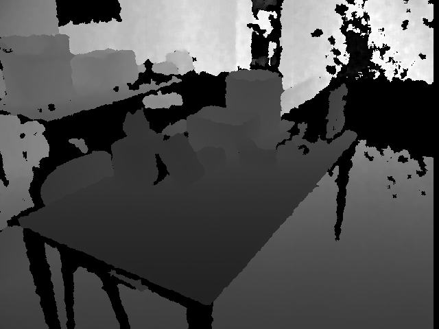
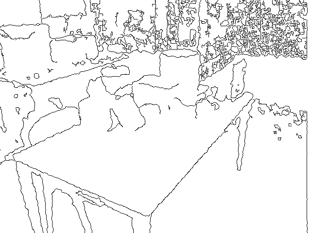
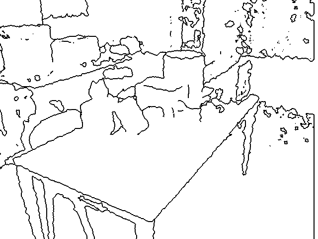
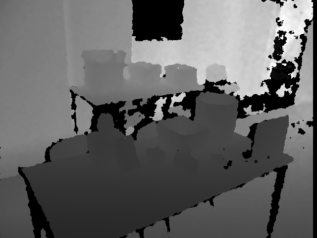
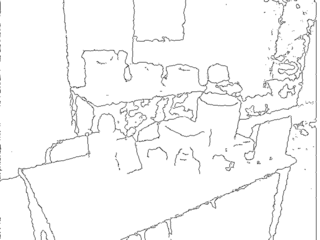
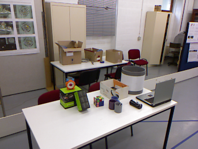
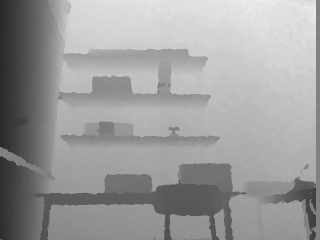
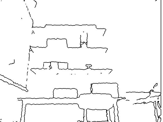
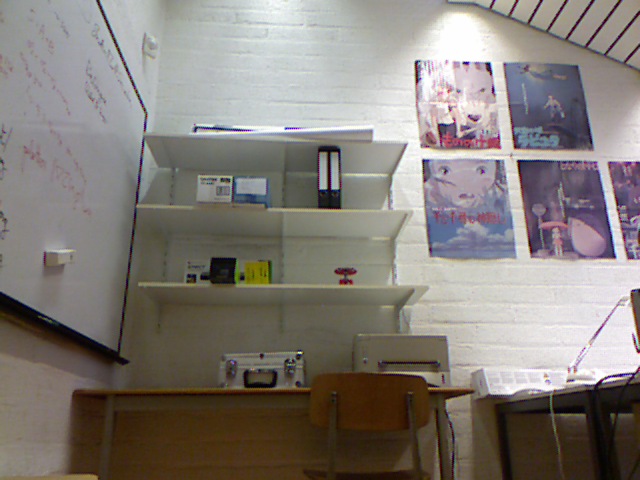
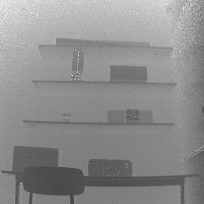
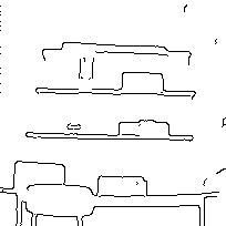
We would have compared our results with other methods or evaluate it with a ground-truth but, to our knowledge, there are no other publications or databases about edge extraction dedicated to the kind of 3D cameras we have considered. Therefore, we only provide qualitative results. In Figures
3↓ and
4↓, we show the results of our edge detector on an indoor scene with a large range of depths. In Figures
5↓ and
6↓, our algorithm is applied on another scene.
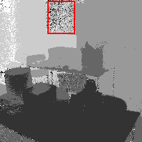
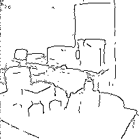
The extracted edges for both cameras reflect the properties of each camera. With the Kinect, the edges follow exactly the detected depth discontinuities as well as the area where the device was unable to compute the depth (black zones in Figure
a↓). It must be noted that, in these zones, the depth is assumed to be zero and thus the standard deviation is also equal to zero. On the contrary, the PMD[vision] CamCube measures depth for every single pixel, some with less confidence than others. We have shown that our criteria provides good results with respect to the value of the amplitude image. For example, in Figure
a↓, despite having some very noisy measurements (indicated by the red rectangle), the edges are relatively well extracted.
The PMD[vision] CamCube camera also has a physical limitation on its maximum depth measurement. Typically, for a 20 Mhz modulation frequency, the maximum range is 7.5 m. Therefore, an edge may be detected at this distance. However, it should be noted that our algorithm behaves as expected for larger distances.
Typical execution time for our algorithm on a Intel Core i7 processor is 15 μs for the Kinect (640 × 480 pixels) and 7 μs for the PMD[vision] CamCube (204 × 204 pixels) with a Gaussian blur with a standard deviation of σfilter = 1.5.
5 Conclusion
We have developed a new jump edge detection algorithm for 3D cameras based on the properties of the devices. Our algorithm is fast and its principle can be adapted to any other 3D sensing device. The Kinect shows better properties than the PMD[vision] CamCube camera for edge detection and thus, its version of the algorithm is more efficient. We have introduced an additional parameter, α. It can be interpreted as the constant of proportionality between the standard deviation of the gradient magnitude and the values used to compute it (squared depth for the Kinect and the amplitude inverse for the PMD[vision] CamCube).
In this paper, we only have detected the jump edges and a roof edge detection technique still needs to be developed for these cameras.
Acknowledgements
A. Lejeune is under a contract funded by the FEDER program of the Walloon Region, Belgium.
6 Appendix: Standard deviation of the derivatives
We define a derivative operator as
Dx(x, y) = ⎲⎳(u, v) ∈ N(x, y)c(u, v)D(u, v),
where
⎧⎪⎨⎪⎩
c(u, v)
≤ 0 ∀u < x
c(x, v)
= 0
c(u, v)
≥ 0 ∀u > x
and
N(x, y) is a neighborhood around the pixel
(x, y) that can be divided between a left neighborhood and a right neighborhood:
∥∇D(x, y)∥adapted = ∥∇D(x, y)∥
− (α)/(∥∇D(x, y)∥)(|Dx(x, y)|(D2(x, y) + D2(x + 1, y))
+ |Dy(x, y)|(D2(x, y) + D2(x, y + 1))) .
Nleft(x, y)
=
{(u, v) ∈ N(x, y)|u < x}
Nright(x, y)
=
{(u, v) ∈ N(x, y)|u > x}.
Without making any assumptions, the standard deviation can be expressed as
[1]:
where
ρ(u, v)(m, n) is the correlation between the pixels
(u, v) and
(m, n).
We will show that the standard deviation is maximum when there is an edge at pixel
(x, y) where we are computing the derivative. Under such circumstances, the correlation between the pixels of the left neighborhood and the pixels of the right neighborhood is zero: the pixels belong to different surfaces. Moreover, if we assume that the pixels of a same surface are correlated (
ρ = 1), the standard deviation becomes
Equation
6↑ contains all the terms of Equation
5↑ where
c(u, v)c(m, n) > 0. Equation
6↑ is thus a superior bound on
σDx(x, y). By triangular inequality, we obtain Equation
4↑.
References
[1] A. Papoulis. Probability, random variables, and stochastic processes. McGraw-Hill, 1991.
[2] B. Parvin, G. Medioni. Adaptive multiscale feature extraction from range data. Computer Vision, Graphics, and Image Proces\-sing, 45(3):346-356, 1989.
[3] B. Steder, R. Rusu, K. Konolige, W. Burgard. Point Feature Extraction on 3D Range Scans Taking into Account Object Boundaries. IEEE International Conference on Robotics and Automation (ICRA), 2011.
[4] J. Canny. A Computational Approach to Edge Detection. IEEE Transactions on Pattern Analysis and Machine Intelligence, 8(6):679-698, 1986.
[5] K. Khoshelham. Accuracy Analysis of Kinect Depth Data. ISPRS Workshop Laser Scanning 2011, XXXVIII-5/W12, 2011.
[6] M. Frank, M. Plaue, H. Rapp, U. Kothe, B. Jahne, F. Hamprecht. Theoretical and experimental error analysis of continuous-wave time-of-flight range cameras. Optical Engineering, 48(1), 2009.
[7] P. Boulanger, F. Blais, P. Cohen. Detection of depth and orientation discontinuities in range images using mathematical morphology. IEEE International Conference on Pattern Recognition (ICPR), 1:729-732, 1990.
[8] R. Krishnapuram, S. Gupta. Morphological methods for detection and classification of edges in range images. Journal of Mathematical Imaging and Vision, 2:351-375, 1992.
[9] S. Coleman, B. Scotney, S. Suganthan. Edge Detecting for Range Data Using Laplacian Operators. IEEE Transactions on Image Processing, 19(11):2814-2824, 2010.
[10] T. Lindeberg. Edge Detection and Ridge Detection with Automatic Scale Selection. International Journal of Computer Vision, 30:117-156, 1998.
[11] X. Jiang, H. Bunke. Edge detection in range images based on scan line approximation. Computer Vision and Image Understanding, 73(2):183-199, 1999.
[12] Z. Xu, R. Schwarte, H. Heinol, B. Buxbaum, T. Ringbeck. Smart pixel —photonic mixer device (PMD)— New system concept of a 3D-imaging camera-on-a-chip. International Conference on Mechatronics and Machine Vision in Practice (M2VIP):259-264, 1998.