Summarizing the performances of a background subtraction algorithm measured on several videos

A. Piérard and M. Van Droogenbroeck
University of Liège
Full paper in PDF

How to cite this reference: A. Piérard and M. Van Droogenbroeck. Summarizing the performances of a background subtraction algorithm measured on several videos. In IEEE International Conference on Image Processing (ICIP), Abu Dhabi, United Arab Emirates, October 2020. [BibTeX entry]

Summary

There exist many background subtraction algorithms to detect motion in videos. To help comparing them, datasets with ground-truth data such as CDNET or LASIESTA have been proposed. These datasets organize videos in categories that represent typical challenges for background subtraction. The evaluation procedure promoted by their authors consists in measuring performance indicators for each video separately and to average them hierarchically, within a category first, then between categories, a procedure which we name “summarization”. While the summarization by averaging performance indicators is a valuable effort to standardize the evaluation procedure, it has no theoretical justification and it breaks the intrinsic relationships between summarized indicators. This leads to interpretation inconsistencies. In this paper, we present a theoretical approach to summarize the performances for multiple videos that preserves the relationships between performance indicators. In addition, we give formulas and an algorithm to calculate summarized performances. Finally, we showcase our observations on CDNET 2014.

Keywords: performance summarization, background subtraction, multiple evaluations, CDNET, classification performance

1 Introduction

A plethora of background subtraction algorithms have been proposed in the literature [15, 17, 16, 14, 13, 1, 11]. They aim at predicting, for each pixel of each frame of a video, whether the pixel belongs to the background, free of moving objects, or to the foreground. Background subtraction algorithms have to operate in various conditions (viewpoint, shadows, lighting conditions, camera jitter, etc). These conditions are covered by different videos in evaluation datasets, such as CDNET [10, 9] or LASIESTA [2].

Measuring the performance on a single video is done at the pixel level, each pixel being associated with a ground-truth class y (either negative c⁻ for the background, or positive c⁺ for the foreground) and an estimated class ŷ (the temporal and spatial dependences between pixels are ignored). Performance indicators adopted in the field of background subtraction are mainly those used for two-class crisp classifiers (precision, recall, sensitivity, F-score, error rate, etc).

To compare the behavior of algorithms, it is helpful to “summarize” all the performance indicators that are originally measured on the individual videos. However, to the best of our knowledge, there is no theory for this summarization process, although an attempt to standardize it has been promoted with CDNET. In CDNET, videos are grouped into 11 categories, all videos in a given category having the same importance, and all categories having also the same importance. In other words, the videos are weighted regardless of their size. The standardized summarization process of CDNET is performed hierarchically by computing an arithmetic mean, first between the videos in a category, then between the categories. This averaging is done for seven performance indicators, one by one, independently. While the procedure of CDNET is valuable, it has two major drawbacks related to the interpretability of the summarized values.

Figure 1 How can we summarize the performances of a background subtraction algorithm, measured on several videos? This figure shows that arithmetically averaging the performances breaks the bijective relationship that exists between the ROC and Precision-Recall (PR) spaces [6]. This paper presents a new summarization technique that guarantees the coherence between any sets of performance indicators.

First, the procedure breaks the intrinsic relationships between performance indicators. The case of the M4CD algorithm, as evaluated on CDNET, topically illustrates this inconsistency. Despite that the F-score is known to be the harmonic mean of precision and recall, the arithmetic mean of the F-scores across all videos is 0.69 while the harmonic mean between the arithmetically averaged precisions and recalls is 0.75. 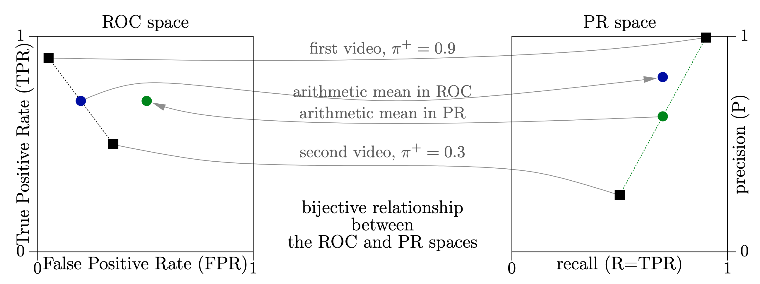The difficulty to summarize F-scores has already been discussed in [4], when averaging between folds in cross-validation. Such a problem also occurs for other indicators. Moreover, Figure 1↑ shows that the summarization with the arithmetic mean breaks the bijective relationship between the ROC and PR spaces [6]. It is not equivalent to summarize the performances in one space or the other. In particular, one could obtain a meaningless arithmetically averaged performance point, located in the unachievable part of the PR space [7] (the achievable part is not convex). This leads to difficulties for the interpretation and, eventually, to contradictions between published summarized results.

Second, some indicators (such as the precision, recall, sensitivity, or error rate) have a probabilistic meaning [3]. Arithmetically averaging these indicators does not lead to a value that preserves the probabilistic meaning. This leads to interpretability issues. Strictly speaking, one cannot think in terms of probabilities unless a random experiment is defined very precisely, as shown by Bertrand’s paradox [5].

This paper presents a better summarization procedure that avoids these interpretability issues. In Section 2↓, we present indicators to measure the performance of an algorithm applied on a single video and pose the random experiment that underpins the probabilistic meaning of these indicators. Then, in Section 3↓, we generalize this random experiment for several videos, and show that the resulting performance indicators can be computed based only on the indicators obtained separately for each video. In other words, we have established a theoretical model for summarization that guarantees a consistency between the indicators resulting from both random experiments. In Section 4↓, we showcase our new summarization procedure on CDNET and discuss how it affects the ranking between algorithms. Section 5↓ concludes the paper.

2 Performance indicators for one video

The performance of a background subtraction algorithm on a video is measured by running it once (even for non-deterministic algorithms), and counting at the pixel level the amounts of true negatives TN (y = ŷ = c⁻), false positives FP (y = c⁻ and ŷ = c⁺), false negatives FN (y = c⁺ and ŷ = c⁻), and true positives TP (y = ŷ = c⁺).

The performance indicators are then derived from these amounts. For example, the prior of the positive class is π⁺ = (FN + TP)/(TN + FP + FN + TP), the rate of positive predictions is τ⁺ = (FP + TP)/(TN + FP + FN + TP), the error rate is ER = (FP + FN)/(TN + FP + FN + TP), the true negative rate (specificity) is TNR = (TN)/(TN + FP), the false positive rate is FPR = (FP)/(TN + FP), the false negative rate is FNR = (FN)/(FN + TP), the true positive rate (recall) is TPR = R = (TP)/(FN + TP), the positive predictive value (precision) is PPV = P = (TP)/(FP + TP), and the F-score is F = (2 TP)/(FP + FN + 2 TP).

The (FPR,  TPR) coordinates define the well-known Receiver Operating Characteristic (ROC) space [12, 18]. The precision P and recall R define the PR evaluation space [7], which is an alternative to the ROC space, as there exists a bijection between these spaces, for a given prior π⁺ [6]. In fact, this bijection is just a particular case of the relationships that exist between the various indicators. There are other famous relationships. For example, the F-score is known to be the harmonic mean of the precision P and recall R.

Despite its importance for the interpretation, it is often overlooked that some indicators have a probabilistic meaning [3]. Let us consider the following random experiment.

Random Experiment 1 (for one video) Draw one pixel at random (all pixels being equally likely) from the video and observe the ground-truth class Y as well as the predicted class Ŷ for this pixel. The result of the random experiment is the pair Δ = (Y, Ŷ).

We use capital letters for Y, Ŷ, and Δ to emphasize the random nature of these variables. The outcome of this random experiment can be associated with a true negative tn = (c⁻, c⁻), a false positive fp = (c⁻, c⁺), a false negative fn = (c⁺, c⁻), or a true positive tp = (c⁺, c⁺). The family of probabilistic indicators can be defined based on this random experiment:

(1) P(Δ ∈ A∣Δ ∈ ℬ) with ∅ ⊊ A ⊊ ℬ ⊆ {tn, fp, fn, tp}

It includes π⁺ = P(Δ ∈ {fn, tp}), τ⁺ = P(Δ ∈ {fp, tp}), ER = P(Δ ∈ {fp, fn}), TNR = P(Δ = tn∣Δ ∈ {tn, fp}), TPR = P(Δ = tp∣Δ ∈ {fn, tp}), and PPV = P(Δ = tp∣Δ ∈ {fp, tp}). All the other performance indicators (the F-score, balanced accuracy, etc) can be derived from the probabilistic indicators.

3 Summarizing the performance indicators for several videos

Let us denote a set of videos by V. We generalize the random experiment defined for one video to several videos as follows.

Random Experiment 2 (for several videos) First, draw one video V at random in the set V, following an arbitrarily chosen distribution P(V). Then, draw one pixel at random (all pixels being equally likely) from V and observe the ground-truth class Y and the predicted class Ŷ for this pixel. The result of the experiment is the pair Δ = (Y, Ŷ).

As the result of this second random experiment is again a pair of classes, as encountered for a single video (first random experiment), all performance indicators can be defined in the same way. This is important for the interpretability, since it guarantees that all indicators are coherent and that the probabilistic indicators preserve a probabilistic meaning.

The distribution of probabilities P(V) parameterizes the random experiment. It can be arbitrarily chosen to reflect the relative weights given to the videos. For example, one could use the weights considered in CDNET. An alternative consists in choosing weights proportional to the size of the videos (the number of pixels multiplied by the number of frames). This leads to identical distributions P(Δ) between the second random experiment and the first one with the fictitiously aggregated video ∪_v ∈ Vv.

Summarization formulas.

We denote by I(v) the value of an indicator I obtained with our first random experiment on a video v ∈ V, and by I(V) the value of I resulting from our second random experiment applied on the set V of videos.

We claim that the indicators I(V) summarize the performances corresponding to the various videos, because they can be computed based on some I(v), exclusively. To prove it, let us consider a probabilistic indicator I_A∣ℬ defined as P(Δ ∈ A∣Δ ∈ ℬ), and I_ℬ as P(Δ ∈ ℬ). Thanks to our second random experiment, we have

(2) I_A∣ℬ(V)  = P(Δ ∈ A∣Δ ∈ ℬ)  = ⎲⎳_v ∈ VP(Δ ∈ A, V = v∣Δ ∈ ℬ)  = ⎲⎳_v ∈ VP(V = v∣Δ ∈ ℬ) P(Δ ∈ A∣Δ ∈ ℬ, V = v)  = ⎲⎳_v ∈ VP(V = v∣Δ ∈ ℬ) I_A∣ℬ(v)\enspace,

with

(3) P(V = v∣Δ ∈ ℬ)  = (P(V = v) P(Δ ∈ ℬ∣V = v))/(P(Δ ∈ ℬ))  = (P(V = v) P(Δ ∈ ℬ∣V = v))/(⎲⎳_{v’ ∈ V}P(V = v’) P(Δ ∈ ℬ∣V = v’))  = (P(V = v) I_ℬ(v))/(⎲⎳_{v’ ∈ V}P(V = v’) I_ℬ(v’)) .

Thus, the summarized probabilistic indicator I_A∣ℬ(V) is a weighted arithmetic mean of the indicators {I_A∣ℬ(v)∣v ∈ V}, the weights being the (normalized) product between the relative importance P(V = v) given to the video v and the corresponding I_ℬ(v):

(4) I_A∣ℬ(V) = ⎲⎳_v ∈ V(P(V = v) I_ℬ(v))/(⎲⎳_{v’ ∈ V}P(V = v’) I_ℬ(v’)) I_A∣ℬ(v).

In the particular case of an unconditional probabilistic indicator I_A = I_{A∣{tn, fp, fn, tp}}, Equation (4↑) reduces to

(5) I_A(V) = ⎲⎳_v ∈ VP(V = v) I_A(v) .

Note that we are able to summarize probabilistic indicators that are undefined for some, but not all, videos. The reason is that I_A∣ℬ(v) is undefined only when I_ℬ(v) = 0, and we observe that only the product of these two quantities appears in Equation (4↑). This product is always well defined since it is an unconditional probability (I_ℬ(v) I_A∣ℬ(v) = I_A∩ℬ(v)). To emphasize it, we rewrite Equation (4↑) as

(6) I_A∣ℬ(V) = ⎲⎳_v ∈ V(P(V = v) I_ℬ(v) I_A∣ℬ(v))/(I_ℬ(V)) = (⎲⎳_v ∈ VP(V = v) I_A∩ℬ(v))/(I_ℬ(V)) = (I_A∩ℬ(V))/(I_ℬ(V)) .

Applying our summarization in the ROC (FPR, TPR) and PR (R = TPR, P = PPV) spaces.

Let us consider the case in which π⁺, τ⁺, FPR, TPR, and PPV are known for each video. The summarized indicators can be computed by Equations (4↑)-(5↑), since π⁺ = I_{fn, tp}, τ⁺ = I_{fp, tp}, FPR = I_{{fp}∣{tn, fp}}, TPR = I_{{tp}∣{fn, tp}}, and PPV = I_{{tp}∣{fp, tp}}. This yields:

(7) π⁺(V)  = ⎲⎳_v ∈ VP(V = v) π⁺(v) ,  τ⁺(V)  = ⎲⎳_v ∈ VP(V = v) τ⁺(v) ,  FPR(V)  = (1)/(π⁻(V))⎲⎳_v ∈ VP(V = v) π⁻(v) FPR(v) ,  TPR(V)  = (1)/(π⁺(V))⎲⎳_v ∈ VP(V = v) π⁺(v) TPR(v) ,  PPV(V)  = (1)/(τ⁺(V))⎲⎳_v ∈ VP(V = v) τ⁺(v) PPV(v) .

The passage from ROC to PR is given by:

(8) PPV(V) = (π⁺(V) TPR(V))/(π⁻(V) FPR(V) + π⁺(V) TPR(V)) .

A generic algorithm for the computation of any summarized indicator.

Let us assume that the elements of the normalized confusion matrix (I_{tn}, I_{fp}, I_{fn}, and I_{tp}) can be retrieved for each video. This could be done by computing them based on other indicators. In this case, an easy-to-code algorithm to summarize the performances is the following:

step 1: arbitrarily weight the videos with P(V),

step 2: retrieve I_{tn}(v), I_{fp}(v), I_{fn}(v), and I_{tp}(v) for each video v,

step 3: then compute I_{tn}(V), I_{fp}(V), I_{fn}(V), and I_{tp}(V) with Equation (5↑),

step 4: and finally derive all the desired summarized indicators based on their relationships with the I_{tn}, I_{fp}, I_{fn}, I_{tp} indicators. For example,

F(V) = (2 I_{tp}(V))/(I_{fp}(V) + I_{fn}(V) + 2 I_{tp}(V)) .

4 Experiments with CDNET 2014

Figure 2 Summarized performances according to two different procedures, in the cropped ROC (upper row) or PR (lower row) spaces, for 36 classifiers evaluated on the CDNET 2014 dataset. The performances obtained by these procedures differ significantly. Only our summarization procedure preserves the bijection between ROC and PR (see text).

We illustrate the summarization with the CDNET 2014 dataset [9] (organized in 11 categories, containing each 4 to 6 videos). We recomputed all the performance indicators for the 36 unsupervised background subtraction algorithms (we could consider all the algorithms as well) whose segmentation maps are given on http://changedetection.net, compared to the ground-truth segmentation maps.

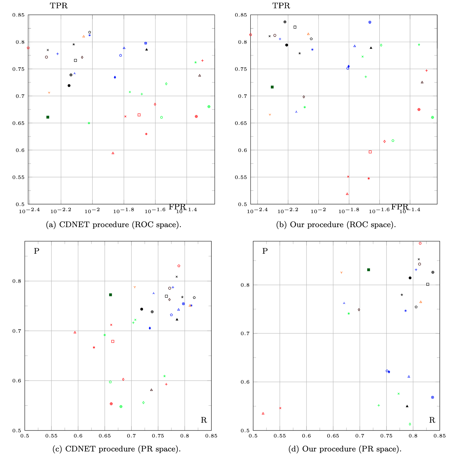
Our first experiment aims at determining if the summarized performance is \strikeout off\xout off\uuline off\uwave offsignificantly\xout default\uuline default\uwave default \strikeout off\xout off\uuline off\uwave offaffected by the summarization procedure\xout default\uuline default\uwave default. Figure 2↑ compares the results of two summarization procedures, in both the ROC and PR spaces.

In the original CDNET procedure, performance indicators are obtained for each category by averaging the indicators measured on each video individually. A final summarized performance is then computed by averaging the performance indicators over the categories.
We applied our summarization, with the same weights for each category as in the original setup; thus, for each video, we have P(V = v) = (1)/(11) × (1)/(M), where M is the number of videos in the corresponding category.

\strikeout off\xout off\uuline off\uwave offIt can be seen that \xout default\uuline default\uwave defaultthe results \strikeout off\xout off\uuline off\uwave offdiffer significantly (both in ROC and PR), which emphasizes the influence of the summarization procedure for the comparison between algorithms. However, with the original summarization procedure, the intrinsic relationships between indicators are not preserved at the summarized level, while ours preserves them.

\strikeout off\xout off\uuline off\uwave offOur second experiment aims at determining if the ranking between algorithms depends on the summarization procedure. Because the F-score is often considered as an appropriate ranking indicator for background subtraction, we performed our experiment with it. Table 1↓\xout default\uuline default\uwave default shows the \strikeout off\xout off\uuline off\uwave offF-scores and ranks obtained according to the same two summarization procedures. We see that the summarization procedure affects the ranking.\xout default\uuline default\uwave default

Algorithm	F of [9]	F (ours)
IUTIS-5	0.7821 (2)	0.8312 (3)
SemanticBGS [8]	0.8098 (1)	0.8479 (1)
IUTIS-3	0.7694 (3)	0.8182 (5)
WisenetMD	0.7559 (4)	0.7791 (10)
PAWCS	0.7478 (8)	0.8272 (4)
SuBSENSE	0.7453 (7)	0.7657 (12)
WeSamBE	0.7491 (6)	0.7792 (9)
SharedModel	0.7569 (5)	0.7885 (8)

Table 1 Extract of F-scores (ranks) obtained with two summarization procedures on CDNET.

5 Conclusion

In background subtraction, algorithms are evaluated by applying them on videos and comparing their results to ground-truth references. Performance indicators of individual videos are then combined to derive indicators representative for a set of videos, during a procedure called “summarization”.

We have shown that a summarization procedure based on the arithmetic mean leads to inconsistencies between summarized indicators and complicates the comparison between algorithms. Therefore, based on the definition of a random experiment, we presented a new summarization procedure and formulas that preserve the intrinsic relationships between indicators. These summarized indicators are specific for this random experiment and for the weights given to the various videos. An easy-to-code algorithm for our summarization procedure has been given. Our procedure is illustrated and commented on the CDNET dataset.

As a general conclusion, for background subtraction involving multiple videos, we recommend to always use our summarization procedure, instead of the arithmetic mean, to combine performance indicators calculated separately on each video. By doing so, the formulas that hold between them at the video level also hold at the summarized level.

References

[1] A. Sobral, A. Vacavant. A comprehensive review of background subtraction algorithms evaluated with synthetic and real videos. Computer Vision and Image Understanding, 122:4-21, 2014. URL https://doi.org/10.1016/j.cviu.2013.12.005.

[2] C. Cuevas, E. Yanez, N. Garcia. Labeled dataset for integral evaluation of moving object detection algorithms: LASIESTA. Computer Vision and Image Understanding, 152:103-117, 2016. URL https://doi.org/10.1016/j.cviu.2016.08.005.

[3] C. Goutte, E. Gaussier. A Probabilistic Interpretation of Precision, Recall and F-Score, with Implication for Evaluation. Advances in Information Retrieval (Proceedings of ECIR), 3408:345-359, 2005.

[4] G. Forman, M. Scholz. Apples-to-apples in Cross-validation Studies: Pitfalls in Classifier Performance Measurement. ACM SIGKDD Explorations Newsletter, 12(1):49-57, 2010.

[5] J. Bertrand. Calcul des probabilités. Gauthier-Villars et fils, 1889.

[6] J. Davis, M. Goadrich. The Relationship Between Precision-Recall and ROC Curves. International Conference on Machine Learning (ICML):233-240, 2006.

[7] K. Boyd, V. Costa, J. Davis, C. Page. Unachievable Region in Precision-Recall Space and Its Effect on Empirical Evaluation. International Conference on Machine Learning (ICML):639-646, 2012.

[8] M. Braham, S. Piérard, M. Van Droogenbroeck. Semantic Background Subtraction. IEEE International Conference on Image Processing:4552-4556, 2017. URL http://www.telecom.ulg.ac.be/publi/publications/braham/Braham2017Semantic.

[9] N. Goyette, P.-M. Jodoin, F. Porikli, J. Konrad, P. Ishwar. A Novel Video Dataset for Change Detection Benchmarking. IEEE Transactions on Image Processing, 23(11):4663-4679, 2014. URL https://doi.org/10.1109/TIP.2014.2346013.

[10] N. Goyette, P.-M. Jodoin, F. Porikli, J. Konrad, P. Ishwar. changedetection.net: A New Change Detection Benchmark Dataset. IEEE International Conference on Computer Vision and Pattern Recognition Workshops (CVPRW), 2012. URL https://doi.org/10.1109/CVPRW.2012.6238919.

[11] N. Vaswani, T. Bouwmans, S. Javed, P. Narayanamurthy. Robust Subspace Learning: Robust PCA, Robust Subspace Tracking, and Robust Subspace Recovery. IEEE Signal Processing Magazine, 35(4):32-55, 2018. URL https://doi.org/10.1109/MSP.2018.2826566.

[12] P. Flach. The Geometry of ROC Space: Understanding Machine Learning Metrics through ROC Isometrics. International Conference on Machine Learning (ICML):194-201, 2003.

[13] P.-M. Jodoin, S. Piérard, Y. Wang, M. Van Droogenbroeck. Overview and Benchmarking of Motion Detection Methods. In Background Modeling and Foreground Detection for Video Surveillance . Chapman and Hall/CRC, Jul 2014. URL http://www.crcnetbase.com/doi/abs/10.1201/b17223-30.

[14] S. Elhabian, K. El-Sayed, S. Ahmed. Moving Object Detection in Spatial Domain using Background Removal Techniques — State-of-Art. Recent Patents on Computer Science, 1:32-54, 2008. URL https://doi.org/10.2174/2213275910801010032.

[15] T. Bouwmans, F. El Baf, B. Vachon. Statistical Background Modeling for Foreground Detection: A Survey. In Handbook of Pattern Recognition and Computer Vision (volume 4) . World Scientific Publishing, January 2010. URL https://doi.org/10.1142/9789814273398_0008.

[16] T. Bouwmans, S. Javed, M. Sultana, S. Jung. Deep Neural Network Concepts for Background Subtraction: A Systematic Review and Comparative Evaluation. Neural Networks, 117:8-66, 2019. URL https://doi.org/10.1016/j.neunet.2019.04.024.

[17] T. Bouwmans. Traditional and recent approaches in background modeling for foreground detection: An overview. Computer Science Review, 11-12:31-66, 2014. URL https://doi.org/10.1016/j.cosrev.2014.04.001.

[18] T. Fawcett. An introduction to ROC analysis. Pattern Recognition Letters, 27(8):861-874, 2006.